|
| Figure 1: A Pattern Diagram |
1.0 Introduction
Aside, perhaps from the above visualization, nothing novel is presented in this post. It follows
an example presented by Freni (1991). I know of this example from problems 7.7 and 7.29 in
Kurz and Salvadori (1995). The oddities of this example can be seen in an earlier and
more complicated example from D'Agata (1983).
This is an example of intensive rent. When the requirements for use are large enough, capitalists will use more than one process
to produce a commodity on homogeneous land. The scarcity of land is expressed in the emergence of rent. This example, though,
is a challenge to Sraffa's work. The cost-minimizing technique is a unique function of the wage, but it is not a unique
function of the rate of profits. The wage frontier is not downward sloping. How disappointing.
2.0 Technology and Requirements for Use
This is an example (Table 1) of a capitalist economy in which one commodity, corn, is produced by laborers working with inputs of (seed)
corn on one type of homogeneous land. Twenty four acres (T = 24) of land are assumed available, and three processes are known
for producing corn
Each process exhibits constant returns to scale (CRS), up to the limit imposed by the
given quantity of land.
Table 1: The Coefficients of Production
| Input | Process |
| I | II | III |
| Labor | a0,1 = 2/5 | a0,2 = 2 | a0,3 = 1 |
| Land | c1,1 = 1/5 | c1,2 = 1/2 | c1,3 = 1/7 |
| Corn | a1,1 = 7/10 | a1,2 = 7/24 | a1,3 = 21/32 |
In this example, requirement for use, also known as net output, is d = 35 bushels. I also take the net output as the numeraire.
3.0 Quantity Flows
I analyze six possible techniques of production. In each of the Alpha, Beta, and Gamma techniques, only one process is used to produce corn.
Table 2 shows the gross output of each process needed to satisfy the requirements for use. Notice the Beta technique requires more land than is
available; it is infeasible.
Table 2: Techniques of Production
| Technique | Process | Acres Used |
| I | II | III |
| Alpha | qα,1 = 350/3 | 0 | 0 | 70/3 ≈ 23.3 |
| Beta | 0 | qβ,2 = 840/17 | 0 | 420/17 ≈ 24.7 |
| Gamma | 0 | 0 | qγ,3 = 1120/11 | 160/11 ≈ 14.5 |
| Delta | qδ,1 = 60 | qδ,2 = 24 | 0 | 24 |
| Epsilon | qε,1 = 3640/29 | 0 | qε,3 = -224/29 | 24 |
| Zeta | 0 | qζ,2 = 4368/95 | qζ,3 = 672/95 | 24 |
In each of the Delta, Epsilon, and Zeta techniques, two processes are applied, side-by-side, in farming the land. Table 2 shows the gross outputs
for these techniques, too. Notice that if the Epsilon technique were adopted, the third process would need to run at a negative level. The
Epsilon process is infeasible.
So for the given technology, acres of land, and requirements for use, the Alpha, Gamma, Delta, and Zeta techniques are feasible. Which
techniques are feasible varies with the requirements for use.
3.1 Alpha Technique
I might as well give some indication of how quantity flows are found. Accordingly, suppose the Alpha technique is adopted.
The gross output of the first process is found by solving the following equation:
d = qα,1 - a1,1 qα,1 = (1 - a1,1) qα,1
The amount of land farmed is c1,1 qα,1. The technique is feasible only if this amount does not
exceed the given amount of land available.
3.2 Delta Technique
On the other hand, suppose the Delta technique is applied. The first process is operated alongside the second process.
The gross outputs of the two processes must be such that
the land is totally farmed:
c1,1 qδ,1 + c1,2 qδ,2 = T
The gross outputs must also be such that the requirements for use are satisfied.
d = (qδ,1 + qδ,2) - (a1,1 qδ,1 + a1,2 qδ,2)
The above is a system of two linear equations in two unknowns, qδ,1 and qδ,2.
Nothing guarantees that in the solution, the levels of gross output must be positive. If they are negative, the technique is infeasible.
4.0 Price Equations
The cost-minimizing technique, at a given rate of profits, depends on prices.
4.1 Alpha Technique
Suppose the Alpha technique is adopted. The land is not fully farmed. Since it is in excess supply, it pays no rent.
The parameters for the first process yield an equation.
pα a1,1 (1 + r) + wα a0,1 = pα
I stated above that net output is the numeraire.
pα d = 1
One can solve the above system to obtain the wage as a function of the rate of profits. The wage curve for the Alpha technique is
downward-sloping.
4.2 Delta Technique
Because of the scarcity of land, a positive rent emerges for the delta technique. The parameters for the two operated processes provide
two equations for the system of prices of production:
pδ a1,1 (1 + r) + ρδ c1,1 + wδ a0,1 = pδ
pδ a1,2 (1 + r) + ρδ c1,2 + wδ a0,2 = pδ
As usual, the specification of the numeraire yields another price equation.
pα d = 1
I want to make a start towards solving the above system. One can multiply the first equation by (1/c1,1), the second
equation by (1/c1,2), and subtract the second from the first:
[a1,1/(dc1,1) - a1,2/(dc1,2)] (1 + r) + wδ[a0,1/c1,1 - a0,2/c1,2] = [1/(dc1,1) - 1/(dc1,2)]
Notice that the rent of land has been eliminated. Land, in Sraffian terminology, is a non-basic commodity. The system of
equations can be solved seperately for the wage and prices as a function of the rate of profits. Then rent can be found afterwards.
This structure also suggests taxing rent of land has no further consequences on the price system.
At least some followers of Henry George should investigate the role of land and non-basic commodities
in post-Sraffian price theory.
5.0 Choice of Technique
Figure 2 graphs the wage curves and rent, for feasible techniques for this example, with the specified requirements for use, against the rate of profits.
For techniques in which two processes are activated on the homogeneous land, the wage curves in the panel on the left are only shown where
rent is non-negative.
|
| Figure 2: Wage Curves and the Frontier |
I indicate the cost-minimizing technique(s) with heavy lines in the above figure. Notice that for a range of profits of approximately 13.3 percent
and 24.7 percent, the Alpha, Delta, and Zeta techniques are all cost-minimizing. The choice of technique is not unique. Furthermore, for a
rate of profits above this range, no technique is cost-minimizing. This result would have been surprising to Sraffa, as I read him.
The wage frontier, in this case, is not the outer frontier of wage curves. Nor is it the inner frontier. So I want to say something
about how the choice of technique is analyzed here.
The wage and the price of corn, as determined by the Alpha technique, can be used to evaluate the costs and revenues, of operating
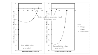
each of the three processes in the technology, at a unit level. The costs include the given rate of profits. The left panel in
Figure 3 shows the difference between such revenues and costs. That is, it shows what are known as extra profits in activating
each process. Notice that no extra profits are to be made in operating the first process, thus confirming that the price
system has been solved correctly. For rates of profits below the first switch point shown, no extra profits can be made
by activating the second or third process; Alpha is cost minimizing in this range. For a higher rate of profits, extra profits
can be made by activating the second process. Alpha is no longer cost-minimizing.
|
| Figure 3: Extra Profits for the Alpha and Gamma Techniques |
The right panel repeats the analysis for the price system for the Gamma technique. For the full range of
feasible rates of profits, no extra profits are obtained by operating the third process, as expected. But
extra profits can always be made, at Gamma prices, by operating the first or second process; Gamma is
never cost-minimizing.
Figure 4 repeats the analysis for the Delta and Epsilon techniques. The costs now include rents.
Only one of three processes available makes extra profits or incurs costs greater than revenues.
The range of the rate of profits in which each of these techniques is cost-minimizing is indicated.
|
| Figure 4: Extra Profits for the Delta and Epsilon Techniques |
6.0 Ricardian Dynamics
The above has shown how to find wage(s), prices, and rent, for a given requirements for use.
Consider the full range of feasible net outputs. Ricardo told a story, using prices of production (not
his terminology) of how the types of land and activated processes vary with an increase in requirements
for use. This story involves wages, population, and his advocacy against the corn laws. Anyway, Figure 1,
at the top of this post, illustrates aspects of Ricardian dynamics in this numeric example.
For a small enough level of net output, land need not be wholly farmed and is in excess supply. The choice of technique can be found by
constructing the outer frontier out of the wage curves for the Alpha, Beta, and Gamma technique. For a small rate of profits, the
Alpha technique is cost-minimizing, while for a larger rate of profits, the Beta technique is cost-minimizing. All wage curves and the
outer frontier are downward-sloping, as in part I of Sraffa (1960).
For a large enough level of net output, but at a still feasible level, the Gamma, Epsilon, and Zeta techniques are the only
feasible techniques. Under Epsilon and Zeta, the first and second processes, respectively, are combined with the third
process so as to ensure that only the amount of land available is farmed. The choice of technique is found from the inner frontier
of the wage curves. For a small rate of profits, the Epsilon technique is cost-minimizing, and the Zeta technique is cost-minimizing
at a high rate of profits. All wage-curves are downward sloping. This example of intensive rent resembles a well-behaved
model of extensive rent.
The difficulties and surprises arise for an intermediate level of net output, as described above.
7.0 Conclusion
I do not fully know what to make of this example. I notice that the cost-minimizing technique is uniquely determined (except
at switch points) by the wage. And it is analyzed by techniques developed by Sraffa and his followers. I can further
apply by approach of perturbing parameters, if I want. Nevertheless, it reveals some of the disappointments arising
from the theory of joint production.
References
- D'Agata, A. 1983. The existence and unicity of cost-minimizing systems in intensive rent theory. Metroeconomica 35: 147-158.
- Freni, G. 1991. Capitale technico nei modelli dinamici ricardiani. Studi Economici, 44: 141-159.
- Kurz and Neri Salvadori. 1995. Theory of Production: A Long-Period Analysis, Cambridge University Press.


