Niall Kishtainy's Pluralist, Popular History Of Economics

This post calls attention to A Little History of Economics, by Niall Kishtainy. Since I only skimmed this in a local bookstore, this post is not a proper review.

Kishtainy's book, in successive chapters, focuses on the lives of specific economists. The concluding chapter asks why one would want to be an economist, a question that is answered, I gather, by the preceding chapters. The book is in the same genre as Robert Heilbroner's The Worldly Philosophers. Since many more economists are covered in a short span, individual chapters are shorter. As I recall, economists (not in this order) covered include:

• Augustine and Thomas Aquinas
• Mercantilists
• Francois Quesnay, Mirabeau, and other Physiocrats
• Adam Smith
• David Ricardo
• Charles Fourier, Robert Owen, and other utopian socialists
• Thomas Malthus
• Friedrich List
• Karl Marx
• William Stanley and Alfred Marshall
• German historical school, Austrian school, and the methodenstreit
• Thorstein Veblen
• Vladimir Lenin and John Hobson
• Ludwig von Mises
• Joan Robinson and Edward Chamberlin
• John Maynard Keynes
• Paul Samuelson, J. R. Hicks
• Friedrich Hayek
• Arthur Lewis, Paul Rosenstein-Rodan, and Raul Prebisch
• Robert Solow, Trevor Swan, and Paul Romer
• Joseph Schumpeter
• Gary Becker
• John Von Neumann and John Nash
• Ken Arrow and Gerard Debreu
• Fidel Castro, Che Guevara, and Andre Frank
• James Buchanan
• Milton Friedman
• George Akerlof and Joseph Stiglitz
• Hyman Minsky
• John Muth, Eugene Fama, and Robert Lucas
• Ed Prescott and Finn Kyland
• Behavioral economics
• Thomas Piketty

Doubtless, if I read the book in detail, I would have objections to specific details. The attempted coverage, however, seems quite impressive. This book extends from before to after most histories. And it covers a wider range of economists than most.

Krugman Confused On Trade, Capital Theory

Over on EconSpeak, Bruce Wilder provides some comments on a post. He notes that economists wanting to criticize glib free-market ideology in the public discourse often seem unwilling to discard neoclassical economic theory.

Paul Krugman illustrates how theoretically conservative and neoclassical a liberal economist can be. (I use "liberal" in the sense of contemporary politics in the USA.) I refer to Krugman's post from earlier this week, in which he adapts an analysis from the theory of international trade to consider technological innovation (e.g., robots). Krugman presents a diagram, in which endowments of capital and labor are measured along the two axes. Krugman does not seem to be aware that one cannot, in general, coherently talk about a quantity of capital, prior to and independently of prices. He goes on to talk about "capital-intensive" and "labor-intensive" techniques of production.

I point to my draft paper, "On the loss from trade", to illustrate my point that one cannot meaningfully talk about the endowment of capital.

(I did submit this paper to a journal. A reviewer said it was not original enough. I emphasized that I was illustrating my points in a flow-input, point output model, with a one-way flow from factors of production to consumption goods, not a model of production of commodities by means of commodities. Steedman & Metcalfe (1979) also has a one-way model, albeit with a point-input, point-output model. So the reviewer's comments were fair. Embarrassingly, I cite other papers from that book. Apparently, I had forgotten that paper, if I ever read it. I suppose that, given the chance, I could have distinguished some of my points from those made in Steedman & Metcalfe (1979). Also, I close my model with utility-maximization; if I recall correctly, Steedman leaves such an exercise to the reader in papers in that book.)

Reference

• Ian Steedman and J. S. Metcalfe (1979). 'On foreign trade'. In Fundamental Issues in Trade Theory (ed. by Ian Steedman).

Reswitching Only Under Oligopoly

Figure 1: Rates of Profits for Switch Points for Differential Rates of Profits

1.0 Introduction

Suppose one knows the technology available to firms at a given point in time. That is, one knows the techniques among which managers of firms choose. And suppose one finds that reswitching cannot occur under this technology, given prices of production in which the same rate of profits prevails among all industries. But, perhaps, barriers to entry persist. If one analyzes the choice of technique for the given technology, under the assumption that prices of production reflect stable (non-unit) ratios of profits, differing among industries, reswitching may arise for the technology. The numerical example in this post demonstrates this logical possibility.

The numerical example follows a model of oligopoly I have previously outlined. In some sense, the example is symmetrical to the example in this draft paper. That example is of a reswitching example under pure competition, which becomes an example without reswitching and capital reversing, if the ratio of the rates of profits among industries differs enough. The example in this post, on the other hand, has no reswitching or capital reversing under pure competition. But if the ratios of the rates of profits becomes extreme enough, it becomes a reswitching example.

2.0 Technology

The technology for this example resembles many I have explained in past posts. Suppose two commodities, iron and corn, are produced in the example economy. As shown in Table 1, two processes are known for producing iron, and one corn-producing process is known. Each column lists the inputs, in physical units, needed to produce one physical unit of the output for the industry for that column. All processes exhibit Constant Returns to Scale, and all processes require services of inputs over a year to produce output of a single commodity available at the end of the year. This is an example of a model of circulating capital. Nothing remains at the end of the year of the capital goods whose services are used by firms during the production processes.

Table 1: The Technology for a Two-Industry Model

Input	Iron Industry		Corn Industry
Labor	1	305/494	1
Iron	1/10	229/494	11/10
Corn	1/40	3/1976	2/5

For the economy to be self-reproducing, both iron and corn must be produced each year. Two techniques of production are available. The Alpha technique consists of the first iron-producing process and the lone corn-producing process. The Beta technique consists of the remaining iron-producing process and the corn-producing process.

3.0 Price Equations

The choice of technique is analyzed on the basis of cost-minimization, with prices of production. Suppose the Alpha technique is cost minimizing. Then the following system of equalities and inequalities hold:

[(1/10)p + (1/40)](1 + rs₁) + w = p

[(229/494)p + (3/1976)](1 + rs₁) + (305/494)w ≥ p

[(11/10)p + (2/5)](1 + rs₂) + w = 1

where p is the price of a unit of iron, and w is the wage.

The parameters s₁ and s₂ are given constants, such that rs₁ is the rate of profits in iron production and rs₂ is the rate of profits in corn production. The quotient s₁/s₂ is the ratio, in this model, of the rate of profits in iron production to the rate of profits in corn production. Consider the special case:

s₁ = s₂ = 1

This is the case of free competition, with investors having no preference among industries. In this case, r is the rate of profits. I call r the scale factor for the rate of profits in the general case where s₁ and s₂ are unequal.

The above system of equations and inequalities embody the assumption that a unit corn is the numeraire. They also show labor as being advanced and wages as paid out of the surplus at the end of the period of production. If the second inequality is an equality, both the Alpha and the Beta techniques are cost-minimizing; this is a switch point. The Alpha technique is the unique cost-minimizing technique if it is a strict inequality. To create a system expressing that the Beta technique is cost-minimizing, the equality and inequality for iron production are interchanged.

4.0 Choice of Technique

The above system can be solved, given s₁, s₂, and the scale factor for the rate of profits. I record the solution for a couple of special cases, for completeness. Graphs of wage curves and a bifurcation diagram illustrate that stable (non-unitary) ratios of rates of profits can change the dynamics of markets.

4.1 Free Competition

Consider the special case of free competition. The wage curve for the Alpha technique is:

w_α = (41 - 38r + r²)/[80(2 + r)]

The price of iron, when the Alpha technique is cost-minimizing, is:

p_α = (5 - 3r)/[8(2 + r)]

The wage curve for the Beta technique is:

w_β = (6,327 - 9,802r + 3,631r²)/[20(1,201 + 213r)]

When the Beta technique is cost-minimizing, the price of iron is:

p_β = [5(147 - 97r)]/[2(1,201 + 213r)]

Figure 2 graphs the wage curves for the two techniques, under free competition and a uniform rate of profits among industries. The wage curves intersect at a single switch point, at a rate of profits of, approximately, 8.4%:

r_switch = (1/1,301)[799 - 24 (826^1/2)]

The wage curve for the Beta technique is on the outer envelope, of the wage curves, for rates of profits below the switch point. Thus, the Beta technique is cost-minimizing for low rates of profits. The Alpha technique is cost minimizing for feasible rates of profits above the switch point. Around the switch point, a higher rate of profits is associated with the adoption of a less capital-intensive technique. Under free competition, this is not a case of capital-reversing.

Figure 2: Wage Curves for Free Competition

4.2 A Case of Oligopoly

Now, I want to consider a case of oligopoly, in which firms in different industries are able to ensure long-lasting barriers to entry. These barriers manifest themselves with the following parameter values:

s₁ = 4/5

s₂ = 5/4

In this case, the wage curve for the Alpha technique is:

w_α = (4,100 - 4,435r + 100r²)/[40(400 + 259r)]

The price of iron, when the Alpha technique is cost-minimizing, is:

p_α = (125 - 96r)/(400 + 259r)

The wage curve for the Beta technique is:

w_β = 8(126,540 - 195,289r + 72,620r²)/[160(24,020 + 9,447r)]

The price of iron, when the Beta technique is cost-minimizing, is:

p_β = 2(3,675 - 3,038r)/(24,020 + 9,447r)

Figure 3 graphs the wage curves for the Alpha and Beta techniques, for the parameter values for this model of oligopoly. This is now an example of reswitching. The Beta technique is cost minimizing at low and high rates of profits. The Alpha technique is cost minimizing at intermediate rates. The switch points are at, approximately, a value of the scale factor for rates of profits of 12.07% and 77.66%, respectively.

Figure 3: Wage Curves for a Case of Oligopoly

4.3 A Range of Ratios of Profit Rates

The above example of oligopoly can be generalized. I restrict myself to the case where the parameters expressing the ratio of rates of profits between industries satisfy:

s₂ = 1/s₁

One can then consider how the shapes and locations of wage curves and switch points vary with continuous variation in s₁/s₂. Figure 1, at the top of this post, graphs the wage at switch points for a range of ratios of rates of profits. Since the Beta technique is cost-minimizing, in the graph, at all high feasible wages and low scale factor for the rates of profits, I only graph the maximum wage for the Beta technique. I do not graph the maximum wage for the Alpha technique.

As the ratio of the rate of profits in the iron industry to rate in the corn industry increases towards unity, the model changes from a region in which the Beta technique is dominant to a reswitching example to an example with only a single switch point. As expected, only one switch point exists when the rate of profits is uniform between industries.

5.0 Conclusion

So I have created and worked through an example where:

• No reswitching or capital-reversing exists under pure competition, with all industries earning the same rate of profits.
• Reswitching and capital-reversing can arise for oligopoly, with persistent differential rates of profits across industries.

No qualitative difference necessarily exists, in the long period theory of prices, between free competition and imperfections of competition. Doubtless, all sorts of complications of strategic behavior, asymmetric information, and so on are empirically important. But it seems confused to blame the failure of markets to clear or economic instability on such imperfections.

Bifurcations in a Reswitching Example

Figure 1: Rates of Profits for Switch Points in One Dimension in Parameter Space

1.0 Introduction

This post presents an example of structural variation in the qualitative behavior of a reswitching example, at different values for selected parameters. I know of few applications of bifurcation analysis to the Cambridge Capital Controversy. Most prominently, I think of Rosser (1983). I suppose I could also point to some of my draft papers. Although not presented this way, one could read Laibman and Nell (1977) as a bifurcation analysis, where the steady state rate of growth is the parameter being varied.

I guess one could read this post as a response to the empirical results in Han and Schefold (2006). Schefold has been developing a theoretical explanation, based on random matrices, of why capital-theoretic paradoxes might be empirically rare. I seem to have stumbled on an explanation of why such paradoxes might arise in practice, and yet might not be observable without more data. To fully address recent results from Schefold, on reswitching and random matrices, one should analyze the spectra of Leontief input-output matrices, which I do not do here.

2.0 Technology

Suppose two commodities, iron and corn, are produced in the economy in the numerical example. As shown in Table 1, two processes are known for producing iron, and one corn-producing process is known. Each column lists the inputs, in physical units, needed to produce one physical unit of the output for the industry for that column. All processes exhibit Constant Returns to Scale, and all processes require services of inputs over a year to produce output of a single commodity available at the end of the year. This is an example of a model of circulating capital. Nothing remains at the end of the year of the capital goods whose services are used by firms during the production processes.

Table 1: The Technology for a Two-Industry Model

Input	Iron Industry		Corn Industry
Labor	1	305/494	a0,2
Iron	1/10	229/494	a1,2
Corn	1/40	3/1976	2/5

Assume a_0,2 is non-negative, and that a_1,2 is strictly positive. For the economy to be self-reproducing, both iron and corn must be produced each year. Two techniques of production are available. The Alpha technique consists of the first iron-producing process and the lone corn-producing process. The Beta technique consists of the remaining iron-producing process and the corn-producing process.

3.0 Choice of Technique

Managers of firms choose the technique to adopt based on cost-minimization. I take a bushel of corn as the numeraire. Assume that labor is advanced, and that wages are paid out of the surplus at the end of the year. For this post, I do not bother setting out equations for prices of production; I have done that many times in the past.

3.1 Reswitching for one Set of Parameter Values

Figure 2 illustrates that this is a reswitching example. This figure is drawn for the following values of the labor coefficient in the process for producing corn:

a_0,2 = 1

The coefficient of production for iron in corn-production, in drawing Figure 2, is set to the following value:

a_1,2 = 2

The economy exhibits capital-reversing around the switch point at an 80% rate of profits.

Figure 2: Wage-Rate of Profits Curves

3.2 Bifurcations with Variations in a Labor Coefficient

Wage-rate of profits curves are drawn for given coefficients of production. And they will be moved elsewhere for different levels of coefficients of production. Consequently, the existence and location of switch points differ, depending on the values for coefficients of production.

Accordingly, suppose all coefficients of production, except a_0,2, are as in the above reswitching example. Consider values of the labor coefficient for corn-production ranging from zero to three. The labor coefficient is plotted along the abscissa in Figure 3. The points on the blue locus in the figure show the rate of profits for the switch points, as a correspondence for the labor coefficient. The maximum rates of profits for the Alpha and Beta techniques are also graphed.

Figure 3: Rates of Profits for Switch Points as One Labor Coefficient Decreases

Figure 3 shows a structural change in the example. Up to a value of a_0,2 of approximately 2.74, this is a reswitching example. For parameter values strictly greater than that, no switch points exist. The maximum rates of profits for the two techniques are constant in Figure 3. The maximum rates of profits are found for a wage of zero, and they do not vary with the labor coefficient. In some sense, only the maximum rate of profits for the Beta technique is relevant in the figure.

3.3 Bifurcations with Variations in a Coefficient of Production for Iron

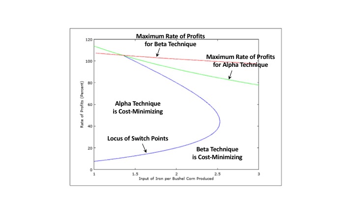
Figure 1, at the top of this post, also shows structural changes. The coefficient of production for iron in corn-production varies in the figure. a_1,2 ranges from one to three. The other coefficients of production are as in the reswitching example in Section 3.1 above. And the blue locus shows the rate of profits at switch points.

The example can seen to have structural variations here, also, with three distinct regions for a_1,2, with the same qualitative behavior in each region. For a low enough value of the coefficient of production under consideration, only one switch point exists. The model remains a reswitching example for an intermediate range of this parameter. And for values of this coefficient of production strictly greater than approximately 2.53, the Beta technique is cost-minimizing for all feasible wages and rates of profits.

The maximum rates of profits, for the Alpha and Beta techniques, are also graphed in Figure 1.

4.0 A Story of Technological Process

Using the above example, one can tell a story of technological progress. Suppose at the start of the story, corn production requires a relatively large input of direct labor and iron, per (gross) unit corn produced. Prices of production associated with this technology are such that only one technique is cost-minimizing. For all feasible wages and rates of profits, firms will want to adopt the Beta technique.

Suppose iron production is relatively stagnant, as compared to corn-production. Innovation in the corn industry reduces the labor and iron coefficients defining the single dominant corn-producing process. After some time, either or both coefficients will be reduced enough that the technology for this economy will have become a reswitching example. And around the switch point at the lower wage (and higher rate of profits), a higher wage is associated with the cost-minimizing technique requiring more labor to be hired, in the overall economy, per given bushel of corn produced (net).

But technological innovation continues to proceed apace. At a even lower coefficient of production for the iron input in the corn industry, the structural behavior of the economy changes again. Now a single switch point exists. And the results of the choice of technique around that switch point conforms to outdated neoclassical intuition.

5.0 Conclusion

This example has two properties that I think worth emphasizing.

The choice of technique in the example corresponds to a choice of a production process in the iron industry. As I have told the story, the technology is fixed in iron production. Innovation occurs in corn production. Thus, innovation in one industry can change the dynamics in another industry.

Second, suppose the technology is observed at a single point of time. Suppose the economy is more or less stationary, and that observation is taken at either the start or the end of the above story. Then neither reswitching nor capital reversing will be observed. Yet such phenomena might arise in the future or have arisen in the past.

References

• David Laibman and Edward J. Nell (1977). Reswitching, Wicksell effects, and the neoclassical production function. American Economic Review. 67 (5): pp. 878-888.
• Zonghie Han and Bertram Schefold (2006). An empirical investigation of paradoxes: reswitching and reverse capital deepening in capital theory. Cambridge Journal of Economics. 30 (5): pp. 737-765.
• J. Barkley Rosser, Jr. (1983). "Reswitching as a cusp catastrophe", Journal of Economic Theory. 31: pp. 182-193.
• Bertram Schefold (2013). Approximate surrogate production functions, Cambridge Journal of Economics. 37 (5): pp. 1161-1184.
• Bertram Schefold (2016). Profits equal surplus value on average and the significance of this result for the Marxian theory of accumulation: Being a new contribution to Engels' Prize Essay Competition, based on random matrices and on manuscripts recently published in the MEGA for the first time. Cambridge Journal of Economics. 40 (1): pp. 165-199.

Here and Elsewhere

• A commentator informs me that the True Levelers revived some ideas put forth in the Peasants Revolt.
• Another commentator points me to Naoki Yoshihara's review of Opocher and Steedman's recent book. Yoshihara has a point, but I think the practice of treating inputs and physically identical outputs as different dated commodities is less applicable in partial models, as opposed to full General Equilibrium. Accountants need guidelines that resist easy manipulation in calculating profits and losses.
• Antonella Palumbo has a post, "Can 'It' Happen Again? Defining the Battlefield for a Theoretical Revolution in Economics", at the Institute for New Economic Thinking. Palumbo argues that a revival of classical economics, without Say's law, can provide an alternative to neoclassical economics. And Keynes' macroeconomics can be usefully be combined with this revival.

A Fluke Switch Point

Figure 1: The Choice of Technique in a Model with Four Techniques

1.0 Introduction

I think I may have an original criticism of (a good part of) neoclassical economics. For purposes of this post, I here define the use of continuously differential production functions as an essential element in the neoclassical theory of production. (This is a more restrictive characterization than I usually employ.) Consider this two-sector example, in which coefficients of production in both sectors varies continuously along the wage-rate of profits frontier. It would follow from this post, I guess, that neoclassical theory is a limit, in some sense, of an analysis in which all switch points are flukes.

I have presented many other, often unoriginal, examples with a continuum of techniques:

• Labor reversing without capital
• Recurrence of capital-output ratio without reswitching
• An example with heterogeneous labor
• Labor demand in a fog
• Slope of 'demand curve' varying with numeraire
• Negative price Wicksell effect, positive real Wicksell effect

I have an example with an uncountably infinite number of techniques along the wage-rate of frontier, but discontinuities for (all?) marginal relationships.

2.0 Technology

I want to compare and contrast two models. The technology in the second model is an example in Salvadori and Steedman (1988).

Households consume a single commodity, called "corn", in both models. In both models, two processes are known for producing corn. And these processes require inputs of labor and a capital good to produce corn. All processes exhibit Constant Returns to Scale, and all processes require services of inputs over a year to produce output of a single commodity available at the end of the year. Both models are models of circulating capital. Nothing remains at the end of the year of the capital goods whose services are used by firms during the production processes.

2.1 First Model

The technology for the first model is shown in Table 1. Each column lists the inputs, in physical units, needed to produce one physical unit of the output for the industry for that column. The two processes for producing corn require inputs of distinct capital goods. One corn-producing process requires inputs of labor and iron, and the other requires inputs of labor and tin.

Table 1: The Technology for a Three-Industry Model

Input	Iron Industry	Tin Industry	Corn Industry
	(a)	(b)	(c)	(d)
Labor	1	2	1	2
Iron	0	0	2/3	0
Tin	0	0	0	1/2
Corn	2/3	1/2	0	0

Two techniques, as shown in Table 2, are available for producing a net output of corn. A choice of a process for producing corn also entails a choice of which capital good is produced. When the processes are each operated on a appropriate scale, the gross output of the process producing the specific capital good exactly replaces the quantity of the capital good used up as an input, summed over both industries operated in the technique.

Table 2: Techniques in a Three-Commodity Model

Technique	Processes
Alpha	a, c
Beta	b, d

2.2 Second Model

The technology for the second model is shown in Table 3. Two processes are known for producing corn. Both corn-producing processes require inputs of labor and iron, but in different proportions.

Table 3: The Technology for a Two-Industry Model

Input	Iron Industry		Corn Industry
	(a)	(b)	(c)	(d)
Labor	1	2	1	2
Iron	0	0	2/3	1/2
Corn	2/3	1/2	0	0

Table 4 lists the techniques available in the second model. The first two techniques superficially resemble the two techniques available in the first model. But, in this model, the first process for producing a capital good can be combined, in a technique, with the second corn-producing producing process. This combination of processes is called the Gamma technique. Likewise, the Delta technique combines the second process for producing a capital good with the first corn-producing processes. Nothing like the Gamma and Delta techniques are available in the first model.

Table 4: Techniques in a Two-Commodity Model

Technique	Processes
Alpha	a, c
Beta	b, d
Gamma	a, d
Delta	b, c

3.0 Prices of Production

Suppose the Alpha technique is cost-minimizing. Prices of production, which permit smooth reproduction of the economy, must satisfy the following system of two equations in three unknowns:

(2/3)(1 + r) + w_α = p_α

(2/3) p_α(1 + r) + w_α = 1

These equations are based on the assumption that labor is advanced, and wages are paid out of the surplus at the end of the year. The same rate of profits are generated in both industries. A unit quantity of corn is taken as the numeraire.

One of the variables in these equations can be taken as exogenous. The first row in Table 5 specifies the wage and the price of the appropriate capital good, as a function of the rate of profits. The equation in the second column is called the wage-rate of profits curve, also known as the wage curve, for the Alpha technique. Table 5 also shows solutions of the systems of equations for the prices of production for the other three techniques in the second model, above. I have deliberately chosen a notation such that the first two rows can be read as applying to either one of the two models.

Table 5: Wages and Prices by Technique

Technique	Wage Curve	Prices
Alpha	wα = (1 - 2 r)/3	pα = 1
Beta	wβ = (1 - r)/4	pβ = 1
Gamma	wγ = 2(2 - 2r - r2) /[3(5 + r)]	pγ = 2(7 + 4r) /[3(5 + r)]
Delta	wδ = (2 - 2r - r2)/(7 + 4r)	pδ = 3(5 + r)/[2(7 + 4r)]

Figure 1, at the top of this post, graphs all four wage-curves. The wage curves for the Alpha and Beta techniques are straight lines. In the jargon, the processes comprising these techniques exhibit the same organic composition of capital. The wage curves for the Gamma and Delta techniques are not straight lines. All four wage-curves intersect at a single point, (r, w) = (20%, 1/5). (The wage curves for the Gamma and Delta techniques have the same intersection with the axis for the rate of profits.)

3.0 Choice of Technique

The cost-minimizing techniques form the outer envelope of the wage curves. For a given wage, the cost minimizing technique is the technique with the highest wage curve in Figure 1. A switch point is a point on the outer envelope at which more than one technique is cost-minimizing. All four wage curves intersect, in the figure, at the single switch point.

The Beta technique is cost-minimizing for wages to the left of the single switch point. The Alpha technique is cost-minimizing for all feasible wages greater than the wage at the switch point. Managers of firms replace both processes in the Alpha technique at the switch point with both processes in the Beta technique.

This is no problem for the first model above. The adoption of a new process for producing corn requires, if the economy is capable of self-replacement before and after the switch, that the process for producing iron or tin be replaced by the process for producing the other.

But consider the other model. For all processes in the Alpha technique to be replaced at a switch point, the wage curves for all techniques composed of all combinations of processes in the Alpha and Beta techniques. In other words, in the second model, wage curves for all four techniques must intersect at the switch point. The example in the second model is a fluke.

I have previously explained what makes a result a fluke, in the context of the analysis of the choice of technique. Qualitative properties, for generic results, continue to persist for some small variation in model parameters.

Consider a model with a discrete number of switch points. Consider the cost-minimizing techniques on both sides of a switch point. And suppose that same commodities are produced in both techniques, albeit in different proportions. Generically, only one process is replaced at such a switch point. All processes, except for that one, are common in both techniques.

5.0 A Generalization to An Uncountably Infinite Number of Processes in Each Industry

Consider a model with more than one industry, but a finite number. Suppose each industry has available an uncountably infinite number of processes. And, in each industry, the processes available for that industry can be described by a continuously differentiable production function. Here I present a two-commodity example with Cobb-Douglas production functions.

There are no switch points in such a model. The cost-minimizing technique varies continuously along the outer-envelope of wage curves. In fact, the processes in each industry, in the cost-minimizing technique varies continuously. Since there are no switch points at all, there is not a single switch point in which more than one process varies, as a fluke, with the cost-minimizing technique.

Nevertheless, cannot one see such "smooth" production functions as a limiting case? If so, it would be a generalization or extension of a discrete model, in which all switch points are flukes, to a continuum. From the perspective of the analysis of the choice of technique in discrete models, typical neoclassical models are nothing but flukes.

6.0 Conclusions

I actually found my negative conclusion surprising. I have tried to be conscious of the distinction between the structure of the two models in Section 2 above. I think at least some examples I have presented cannot be attacked by the above critique. They are examples of the first, not the second model. I tend to read Samuelson (1962) in the same way, as not sensitive to the critique in this post.

References

• Neri Salvadori and Ian Steedman (1988). No reswitching? No switching! Cambridge Journal of Economics, V. 12: pp. 481-486.
• Samuelson, P. A. (1962). Parable and Realism in Capital Theory: The Surrogate Production Function, V. 29, No. 3: pp. 193-206.
• J. E. Woods 1990. The Production of Commodities: An Introduction to Sraffa, Humanities Press International.

Bifurcations Of Roots Of A Characteristic Equation

Figure 1: Rates of Profits for Beta Technique

I have previously considered all roots of a polynomial equation for the rate of profits in a model, of the choice of technique, in which each technique is specified by a finite series of dated labor inputs. One root is the traditional rate of profits, but there are uses for the other roots:

• All roots appear in an equation defining the Net Present Value (NPV) for the technique, given the wage and the rate of profits.
• All roots can be combined in an accounting identity for the difference between labor commanded and labor embodied, given the wage.

I thought it of interest to know whether these non-traditional roots are real or complex, as they vary with the wage. I am considering multiple roots in an attempt to build on and critique Michael Osborne's approach to multiple interest rate analysis.

I also have considered examples of models of the production of commodities by means of commodities, in which at least one commodity is basic, in the sense of Sraffa. And I have attempted to apply or extend my critique of multiple interest rate analysis to these models. The point of this post is to illustrate possibilities on the complex plane for multiple interest rates in these models.

A technique in models of the production of commodities by means of commodities, as least in the case when all capital is circulating capital, is specified as a vector of labor coefficients and a Leontief input-output matrix. In parallel with my approach to techniques specified by a finite sequence of dated labor inputs, consider wages as being advanced - that is, not paid at the end of the year out of the surplus - in such models. Given the wage and the numeraire, one can construct a square matrix in which each coefficient is the sum of the corresponding coefficient in the Leontief input-output matrix and the quantity of the commodity produced by that industry that is advanced to the workers, per unit output produced. I call this matrix the augmented input-output matrix.

A polynomial equation, called the characteristic equation, is solved to find eigenvalues of the augmented input-output matrix. The power of this polynomial is equal to the number of commodities produced by the technique. The number of roots for the polynomial is therefore equal to the number of commodities. A rate of profits corresponds to each root. Assume the Leontief input-output matrix is a Sraffa matrix and that the wage does not exceed a certain maximum. Under these conditions, the Perron-Frobenius theorem picks out the maximum eigenvalue of the augmented input-output matrix. The corresponding rate of profits is non-negative, and the prices of production of these commodities are positive at the given wage. I was not able to find an application for the other, non-traditional rates of profits.

I present a numerical example in this working paper. This is a three-commodity example with two techniques. Figure 1 graphs the three roots, at different level of wages, for the Beta technique in that example.

In a previous blog post, I extend that example such that managers of firms have a choice of process for producing each of the three commodities. As a consequence, a choice among eight techniques arises. And one can draw a graph like Figure 1 for each technique in that example. Figure 2 shows the corresponding graph for the Delta technique.

Figure 2: Rates of Profits for Delta Technique

In Figures 1 and 2, the rate of profits picked out by the Perron-Frobenius theorem and used to draw the wage-rate of profits curve for the technique lies along the line segment on the real axis on the left in the figure. A lower wage corresponds to a higher traditional rate of profits. Thus, points further to the right on this line segment correspond to a lower wage. A wage of zero leads to the right-most point on this line segment. The highest feasible wage corresponds to left-most point, at a rate of profits of zero, on this segment.

Two non-traditional rates of profits arise for the other two solutions of the characteristic equation. They are plotted to the right on the graphs in Figures 1 and 2. When complex, they are complex conjugates. I thought it of interest that, in Figure 2, they are purely real for two non-overlapping, distinct ranges of feasible levels of the wage.

I draw no practical, applied implications from the non-traditional rates of profits. I just think the graphs are curious.

Some Obituaries for Kenneth Arrow

Bill Black has one here, emphasizing Arrow's impossibility theorem. The blog, A Fine Theorem, has two of a planned four-part series. The first is on the impossibility theorem. The second is about General Equilibrium. The two planned, I gather, are to be about learning-by-doing and health economics, respectively.

I have written several posts drawing on Arrow's work. This one, on a sophisticated neoclassical response to the Cambridge Capital Controversy, is among my most popular posts.

A Reswitching Example in a Model of Oligopoly

The Roots of a Cubic Polynomial Defining Switch Points

I have a draft paper up at SSRN. The abstract:

This paper illustrates, through a numerical example of reswitching under oligopoly, the existence of implications from the Cambridge Capital Controversy for the theory of industrial organization. Oligopoly is modeled by given and persistent ratios in rates of profits among industries, as expressed in a system of equations for prices of production. The numerical example illustrates that this model of oligopoly is a pertubation of free competition. Some comparisons and contrasts are drawn to a model of free competition.

In some sense, this paper shows a somewhat more comprehensive description of value through exogenous distribution than in Sraffa's book. The model can depict capitalists as squabbling over the division of the surplus that their class gets, as well as their struggle against the workers. I'd like to see an example of reswitching or capital reversing in this model, with all (price and real) Wicksell effects as negative in the example in the special case of free competition. I do not see why one cannot arise. Such an example would suggest that "perverse" examples can obtain empirically, even if they are not found in an analysis that presumes one common rate of profits among all industries.

The graph at the top of this post does not appear in the paper. In the model, the ratios of rates of profits among industries are given parameters. A cubic polynomial is defined for a given set of such ratios. Non-negative, real zeroes of that polynomial below a certain maximum define a scale factor for switch points. The location of the zeros varies with the ratios. I happen to be able to solve for the zeros. They are shown in the graph above.

Festschrifts for Sraffians

We are on, maybe, the third generations of Sraffians. An annoyance and a delight of publicly taking up a topic is that one must continually read advances, whether large or small, in your topic. I've read some festschrifts over the last several decades:

• Competing Economic Theories: Essays in memory of Giovanni Carvale, edited by Serio Nisticó and Domenico Tosato.
• Value, Distribution and Capital: Essays in honour of Pierangelo Garegnani, edited by Gary Mongiovi and Fabio Petri.
• Economic Theory and Economic Thought: Essays in Honour of Ian Steedman, edited by John Vint, J. Stanley Metcalfe, Heinz D. Kurz, Neri Salvadori, and Paul A. Samuelson.

I'm aware of some I have not read:

• Social Fairness and Economics: Essays in the spirit of Duncan Foley, edited by Lance Taylor, Armon Rezai, and Thomas Michl.
• Keynes, Sraffa and the Criticism of Neoclassical Theory: Essays in honour of Heinz Kurz, edited by Neri Salvadori and Christian Gehrke.
• Classical Political Economy and Modern Theory: Essays in honour of Heinz Kurz, edited by Christian Gehrke, Neri Salvadori, Ian Steedman and Richard Sturn.
• Economic Theory and its History, edited by Guiseppe Freni, Heinz D. Kurz, Andrea Mario Lavezzi, and Rudolfo Signorino. (This apparently is a celebration of Neri Salvadori's work.)
• Production, Distribution and Trade: Essays in honour of Sergio Parrinello, edited by Adriano Birolo, Duncan K. Foley, Heinz D. Kurz, Bertram Schefold and Ian Steedman
• The Evolution of Economic Theory: Essays in honour of Bertram Schefold, edited by Volker Caspari.

This post provides another demonstration that at least one school of heterodox economists looks, from the outside, like any other group of academics with common research interests. I have posted about Post Keynesianism in this respect. Likewise, I once listed textbooks.

A Story Of Technical Innovation

Figure 1: The Choice of Technique in a Model with Four Techniques

1.0 Introduction

I often present examples of the choice of technique as an internal critique of neoclassical economics. The example in this post, however, is closer to how I think techniques evolve in actually existing capitalist economies. Managers of firms know a limited number of processes in each industry, sometimes only the one in use. Accounting techniques specify a set of prices. An innovation provides a new process in a given industry. The first firm to adopt that process may obtain supernormal profits, whatever the wage or normal rate of profits. Other firms will strive to move into the industry with supernormal profits and to use the new process. Prices associated with the new technique result in the wage-rate of profits frontier being moved outward, perhaps along its full extent.

This example was introduced by Fujimoto (1983). I know it most recently from problem 22 in Woods (1990: p. 126). It is also a problem in Kurz and Salvadori (1995). Fujimoto probably labels it a curiosum because of details more specific than the above overview of how Sraffians might treat technical change.

2.0 Technology

This example is a two-commodity model, in which both commodities, called iron and corn, are basic. Suppose iron is used exclusively as a capital good, and corn is used for both consumption and as a capital good. Consider the processes shown in Table 1. Each process exhibits Constant Returns to Scale. The coefficients in each column show required inputs, per unit output, in each industry for each process. Each process requires a year to complete, and outputs become available at the end of the year. This is a circulating capital model. All commodity inputs are totally used up in the year by providing their services during the course of the year.

Table 1: The Technology

Input	Iron Industry		Corn Industry
	(a)	(b)	(c)	(d)
Labor	1/2	1/10	1/2	3/5
Iron	0	0	2/5	1/5
Corn	2/5	1/10	0	0

For this economy to be reproduced, both iron and corn must be (re)produced. A technique consists of an iron-producing and a corn-producing process. Table 2 lists the four techniques that can be formed from the processes listed in Table 1. In this example, not all processes or techniques are known at the start of the dynamic process under consideration.

Table 2: Techniques

Technique	Processes
Alpha	a, c
Beta	a, d
Gamma	b, c
Delta	b, d

3.0 Price Systems

A system of prices of production characterize smooth reproduction with a given technique. Suppose a unit of corn is the numeraire. Let w be the wage, r be the (normal) rate of profits, and p be the price of a unit of iron. Suppose labor is advanced, and wages are paid out of the surplus. If the Alpha technique is in use, prices of production satisfy the following system of two equations in three unknowns:

(2/5)(1 + r) + (1/2) w = p

(2/5) p (1 + r) + (1/2) w = 1

A non-negative price of iron and wage can be found for all rates of profit between zero and a maximum associated with the technique. Figure 1 illustrates one way of depicting this single degree of freedom, for each technique.

4.0 Innovations

I use the above model to tell a story of technological progress. Suppose at the start, managers of firms only know one process for producing iron and one process for producing corn. Let these be the processes comprising the Alpha technique. In this story, the rate of profits is exogenous, at a level below the rate of profits associated with the switch point between the Gamma and Delta technique, not that that switch point is relevant at the start of this story.

Somehow or other, prices of production provide a reference for market prices. For such prices, the economy is on the wage-rate of profits curve for the Alpha technique in Figure 1. This curve is closest to the origin in the figure.

Suppose researchers in the corn industry discover a new process for producing corn, namely process (d). A choice of technique arises. Corn producers see that they can earn extra profits by adopting this technique at Alpha prices. The Beta technique becomes dominant. Eventually, the extra profits are competed away, and the economy lies on the wage-rate of profits curve for the Beta technique. Under the assumption of an externally specified rate of profits, the wage has increased.

Next, an innovation occurs in the iron industry. Firms discover process (b). At Beta prices, it pays for iron-producing firms to adopt this new process. The wage-rate of profits curve for the Delta technique lies outside the wage-rate of profits curve for the Beta technique. Thus, the Delta technique dominates the Beta technique. But prices of production associated with the Delta technique cannot rule. If the Delta technique were prevailing, corn-producing firms would find they can earn extra profits by discarding process (d) and reverting to process (c). The Gamma technique is dominant at the given rate of profits, and workers will end up earning a still higher wage.

I guess this story does not apply to the United States these days. In the struggle over the increased surplus provided by technological innovation, workers do not seem to be gaining much. At any rate, Table 3 summarizes the temporal sequence of the dominant technique in this story.

Table 3: A Temporal Series of Innovations

Events	Dominant Technique	Processes in Use
Processes (a) and (c) known	Alpha	a, c
Processes (d) introduced	Beta	a, d
Process (b) introduced	Gamma	b, c

I do not see why one could not create an example with a single switch point between the Gamma and Delta techniques, where that switch point is at a wage below the maximum wage for the Alpha technique. For such a postulated example, one could tell story, like the above, with a given wage. The capitalists would end up with all the benefits from technological progress.

5.0 Conclusion

This example illustrates that innovation in one industry (that is, the production of iron) can result in the managers of firms in another industry (corn-production) discarding a previously introduced innovation and reverting to an old process of production.

References

• T. Fujimoto 1983. Inventions and Technical Change: A Curiosum, Manchester School, V. 51: pp. 16-20.
• Heinz D. Kurz and Neri Salvadori 1995. Theory of Production: A Long Period Analysis, Cambridge University Press.
• J. E. Woods 1990. The Production of Commodities: An Introduction to Sraffa, Humanities Press International.

A Model Of Oligopoly

1.0 Introduction

Suppose barriers to entry exist in an economy. Entrepreneurs and capitalists find that they cannot freely enter or exit some industries. And these barriers are manifested by stable ratios of rates of profits among industries. This post presents equations for prices of production under these assumptions.

I suggest that the model presented here fits into the tradition of Old Industrial Organization, as formulated by Joe Bain and Paolo Sylos Labini. As I understand it, Sylos Labini may have once written down equations like these, but never presented them or published them. I suppose this model is also related to work Piero Sraffa published in the 1920s.

2.0 The Model

Consider an economy consisting of n industries. Suppose the rate of profits in the jth industry is (s_j r), where r is the base rate of profits, s_j is positive, and:

s₁ + s₂ + ... + s_n = 1

For simplicity, I limit my attention to a circulating capital model of the production of commodities by means of commodities. For the technique in use, let a_{i, j} be the quantity of the ith commodity used to produce a unit of output in the jth industry. Homogeneous labor is the only unproduced input in each industry. Let a_{0, j} be the person years of labor used to produce a unit output in the jth industry. I assume labor is advanced, and wages are paid out of the surplus at the end of production period, say, a year. Then prices of production, which ensure a smooth reproduction of the economy, satisfy the following system of equations:

(a_{1, 1} p₁ + a_{2, 1} p₂ + ... + a_{n, 1} p_n)(1 + s₁ r) + w a_{0, 1} = p₁

(a_{1, 2} p₁ + a_{2, 2} p₂ + ... + a_{n, 2} p_n)(1 + s₂ r) + w a_{0, 2} = p₂

. . .

(a_{1, n} p₁ + a_{2, n} p₂ + ... + a_{n, n} p_n)(1 + s_n r) + w a_{0, n} = p_n

The coefficients of production, including labor coefficients, and the ratios of the rate of profits are given parameters in the above system of equations. The unknowns are the prices, the wage, and the base rate of profits. Since only relative prices matter in this model, one degree of freedom is eliminated by choosing a numeraire:

p₁ q^*₁ + ... + p_n q^*_n = 1

Since there are n price equations, appending the above equation for the specified numeraire yields a model with (n + 1) equations and (n + 2) unknowns. One degree of freedom remains.

3.0 In Matrix Form

The above model can be expressed more concisely in matrix form. Define:

• I is the identity matrix.
• e is a column vector in which each element is 1.
• S is a diagonal matrix, with s₁, s₂, ..., s_n along the principal diagonal.
• p is a row vector of prices.
• q^* is the column vector representing the numeraire.
• A is the Leontief input-output matrix, representing the technique in use.
• a₀ is the row vector of labor coefficients for the technique.

The model consists of the following equations:

e^T S e = 1

p A (I + r S) + w a₀ = p

p q^* = 1

4.0 Conclusion

One could develop the above model in various directions. For example, one could plot the wage-base rate of profits curve for the technique in use. Of interest to me would be presenting examples of the choice of technique, including reswitching and capital-reversing. The Sraffian critique of neoclassical economics is not confined to the theory of perfect competition.

Update (16 January 2017): I find I have outlined this model before.

Reswitching In An Example Of A One-Commodity Model

Figure 1: The Choice of Technique in a Model with One Commodity

1.0 Introduction

This post presents a reswitching example in a one-good model. The single produced commodity in the example can be used as both a consumption and a capital good. It is produced by expenditure of labor with its services. It lasts for three production periods, and its technical efficiency varies over the course of its lifetime, when used as a capital good.

I do not remember any comparable numeric example in the literature. If I recall Ian Steedman's 1994 article, he gives instructions for constructing a one-good example, but does not present one. Maybe if I reread it now, I will find it clearer. I have previously worked through a reswitching example, with fixed capital, from J. E. Woods. But that is a multi-commodity model. I have also once echoed Sraffa's analysis of depreciation charges, in a case with constant efficiency.

2.0 Technology

This is an example of fixed capital, a kind of joint production. Three production processes are known by the manager of firms, and they each exhibit constant returns to scale. Each process requires a year to complete, and each process produces new widgets. Table 1 shows the inputs for each process, when operated at a unit level, and Table 2 shows the outputs. For example, process I requires inputs of labor and new widgets. The outputs of process I consist of new widgets and the widgets which provided their services throughout the year it is under operation. Those leftover widgets are one year older, though. Consumers consume new widgets during the year following on their purchase. The physical life of widgets, when providing services for production, is three years. Thus, three processes can be operated in production.

Table 1: Inputs for The Technology

Input	Process
	(I)	(II)	(III)
Labor	10	60	13/2
New Widgets	1/3	0	0
One-Year Old Widgets	0	1/3	0
Two-Year Old Widgets	0	0	1/3

Table 1: Outputs for The Technology

Output	Process
	(I)	(II)	(III)
New Widgets	1	7/12	79/20
One-Year Old Widgets	1/3	0	0
Two-Year Old Widgets	0	1/3	0

Firms are not required to operate all three processes. They can truncate the use of widgets after one or two years. Assume free disposal, that is, that discarding widgets does not incur a cost. Under these assumptions, three techniques are available to produce new widgets, as shown in Table 3.

Table 3: Techniques

Technique	Processes
Alpha	I
Beta	I, II
Gamma	I, II, II

3.0 Price Equations

Managers of widget-producing firms choose the technique, that is, the truncation period, on the basis of cost. As usual, consider a competitive economy, in which workers and firms are free to seek out higher wages and profits, respectively. Revenues and costs are calculated on the basis of a set of prices in which workers and firms have no incentive to move out of one process and into another. Workers receive a common wage of w new widgets per person-year. Assume workers are paid out of the surplus at the end of each year. Firms receive a rate of profits of 100 r percent in operating each process in use. For notational convenience, define R:

R = 1 + r

Let p₁ be the price of a one-year old widget and p₂ the price of a two-year old widget.

I confine the systems of price equations for the Alpha and Beta techniques to an appendix. Accordingly, assume the Gamma technique is in use. The wage, prices, and the rate of profits must satisfy a system of three equations:

(1/3)R + 10 w = 1 + (1/3) p₁

(1/3) p₁ R + 60 w = 7/12 + (1/3) p₂

(1/3) p₂ R + (13/2) w = 79/20

Given the rate of profits below some maximum, one can solve for the wage:

w_γ = (60 R² + 35 R + 237 - 20 R³)/(10 (60 R² + 360 R + 39))

The price of two-year old and one-year old widgets fall out:

p_{2, γ} = (237 - 390 w_γ)/(20 R)

p_{1, γ} = (7 + 4 p_{2, γ} - 720 w_γ)/(4 R)

If you feel like it, you can substitute on the Right Hand Sides of the above two equations so as to express prices as functions exclusively of the rate of profits.

4.0 Choice of Technique

I have explained above how to find the wage, as a function of the rate of profits, when the Gamma technique is in use. The wage-rate of profits curves for the Alpha and Beta technique are, respectively:

w_α = (3 - R)/30

w_β = (12 R + 7 - 4 R²)/(120 (R + 6))

Figure 1 graphs all three wage curves. The cost-minimizing technique, at any given rate of profits, is the technique on the outer envelope of the wage curves. The switch points between the Alpha and Gamma techniques are at rates of profits of 10% and 50%. Below 10% and above 50%, the Gamma technique is cost-minimizing. Widgets are used in production processes to the extent of their physical life. Between these rate of profits, the Alpha technique is cost minimizing. The use of widgets, as capital goods, is truncated after one year. For what it is worth, the switch point between the Alpha and Beta techniques, within the outer envelope, is at a rate of profits of 41/24, approximately 171%.

4.1 A Direct Method with Alpha Prices

In the general theory of joint production, an analysis of the choice of technique cannot generally be based on wage-rate of profits curves. Such an analysis does work in this model of fixed capital. But I checked it with a more direct method of analysis.

Suppose the Alpha technique is in use. The prices of one-year old and two-year old widgets are zero. The wage is as found from the system of price equations associated with the Alpha technique. Would it pay to produce new widgets with one-year old or two-year old widgets? Figure 2 shows calculations to determine if supernormal profits can be earned with the Beta or Gamma technique.

Figure 2: Supernormal Profits at Alpha Prices

Since the Alpha technique is in use, its net present value is zero. Extra profits are assumed to have been competed away.

If the Beta technique is operated, no extra profits or losses are earned in operating process I under the Beta technique. In operating process II, the services of old widgets are free, and no revenues are received for the two-year old widgets disposed of at the end of the year. At low rates of profits and high wages, the revenues received for new widgets produced with process II do not cover labor costs. At high rates of profits, the opposite is the case. These prices, when wages are low, signal to firms that they can earn extra profits by extending the truncation period one year.

The analysis for the Gamma technique is more cumbersome. Firms can not adopt process III without also operating process II. Accordingly, the net present value for the Gamma technique is found by accumulating all costs and revenues for all three processes to the end of the third year. In such a weighted sum, the revenues for process I are multiplied by (1 + r)², and the revenues for process II are multiplied by (1 + r). At a rate of profits below 10% and above 50%, firms will want to adopt the Gamma technique and produce with old widgets to the end of their physical life.

4.2 A Direct Method with Beta Prices

I find of interest some complications that arise in applying this direct method with wages and prices, as calculated for the Beta price system. Figure 3 shows the net present value for the processes comprising each of the three techniques. At all rates of profits, these prices signal that firms should extend the truncation period, from two years, to the three years specified by the Gamma technique. This is so, even for rates of profits between 10% and 50%. If firms start at a two-year truncation period, they will only find that they need to truncate to one year after first extending production to three years. (See A.3 in the Appendix for graphs associated with the Gamma price system.)

Figure 3: Supernormal Profits at Beta Prices

When the Beta technique is operated, a price must be assigned to the price of a one-year old widget. In the theory of joint production, prices can be negative when calculated for rates of profits below the maximum. (This is not so for pure circular capital models without joint production.) Figure 4 graphs the price of one-year old widgets, under the system of prices associated with the Beta technique. This price is negative for rates of profits of approximately 171%. Confine your attention to the Alpha and Beta techniques for a second. The negative price of one-year old widgets signals firms that it is profitable to truncate production from two years to one year.

Figure 4: Price of One-Year Widget with Beta Technique

The application of a direct method for comparing costs and revenues for techniques of production confirms, in the context of this model of fixed capital, the results of constructing the outer envelope curve from the wage-rate of profits curves for the techniques.

5.0 Conclusion

The literature on macroeconomics contains many models with aggregate production functions and in which the one produced commodity can be either consumed by households or used as a capital good in further production. And, in many of these models, this capital good depreciates over many periods. These models are one-good models, in the sense of this post. Some mainstream economists ignorantly assert that the Cambridge Capital Controversy was exclusively about problems in aggregating capital goods. Since mainstream economists are aware of aggregation issues, they somehow conclude they are justified in ignoring the controversy. I usually refute this rot by pointing out consequences for microeconomics of the analysis of the choice of technique. This post takes an alternative approach. It examines a highly aggregated model. And issues related to Sraffa effects arise in the one-good model, too.

This example also has a bearing on a misunderstanding common among the Austrian school of economics. Böhm Bawerk, at least, thought of production processes taking a longer amount of time as being more capital intensive and, therefore, more productive, in some sense. Firms are supposedly restricted in how willing they are to temporally extend production processes because of the scarcity of capital, as reflected in the interest rate. If households were less impatient and more willing to save, the interest rate would fall and firms would adopt longer processes. One can find many Austrian school economists (for example, Hayek in the 1930s) rejecting the idea that there exists a meaningful quantitative measure of roundaboutness or the period of production, whether independent of prices or not. But Austrian school economists generally retain a sense that the theory is insightful and somehow qualitatively true. The numeric example challenges this idea. One would think that a truncation of the production process, with the capital good not reaching its physical lifetime, is unambiguously less roundabout. As noted in Figure 1, for one switch point in the example, such a truncation can be associated with a lower interest rate.

Appendix A

I confine various mathematical details to this appendix.

A.1 Alpha Price Equations

If the Alpha technique is in use, the prices of one-year old and two-year old widgets is zero:

p_{1, α} = p_{2, α} = 0

The wage and the rate of profits are related by the coefficients of production for process I:

(1/3)R + 10 w = 1

The wage, under the Alpha technique, can be expressed as a function of the rate of profits, as illustrated in Figure 1.

A.2 Beta Price Equations

If the Beta technique is in use, the price two-year old widgets is zero:

p_{2, β} = 0

A system of two equations arises for the Beta technique:

(1/3)R + 10 w = 1 + (1/3) p₁

(1/3) p₁ R + 60 w = 7/12

The wage as a function of the rate of profits, for the Beta technique, is also illustrated above. The price of one-year old widgets is:

p_{1, β} = R + 30 w_β - 3

A.3 Direct Method with Gamma Prices

This section presents two graphs with wages and the rate of profits found from the system of prices for the Gamma technique. Figure 5 shows the net present value of truncating the use of widgets after one, two, or three years. For all techniques, revenues and costs are accumulated, at the going rate of profits to the end of the last year in which widgets are produced with the technique. The net present value for operating the Alpha technique (truncating after one year) is positive between the switch points at rates of profits of 10% and 50%.

Figure 5: Supernormal Profits at Gamma Prices

Figure 6 shows the prices of one-year old and two-year old widgets for the solution to the Gamma price system. Although not very easy to see in the graph, the price of one-year old widgets is negative at rates of profits between 10% and 50%.

Figure 6: Price of Widgets with Gamma Technique

References

• Ian Steedman. 1994. 'Perverse' Behaviour in a 'One Commodity' Model. Cambridge Journal of Economics, V. 18, No. 3: pp. 299-311.

On Ajit Sinha On Sraffa

Over at the Institute for New Economic Theory (INET), Ajit Sinha discusses the Sraffian revolution. Scott Carter cautions that, in interpreting Sraffa's thought, his archives have barely been touched.

Sinha's article has this blurb, with which I entirely agree:

"The prominence of the debate over 'reswitching' has obscured the importance of Piero Sraffa's profound contribution to economics. It's time to revisit and build on that body of work."

One can agree with the above without following Sinha very far. In analyzing the choice of technique, I often point out more than reswitching. I try to find effects in other markets than the capital markets and go in other directions. Since my motivation for working through these examples is frequently an internal criticism of neoclassical economics, I am frequently willing to assume Constant Returns to Scale and perfect competition, in the sense that firms take prices as given. One might argue that this misses Sraffa's point. Besides one can use 'reswitching' as a synecdoche for such analyses of the choice of technique.

How do I know that Production of Commodities by Means of Commodities: Prelude to a Critique of Economic Theory was about more than Sraffa effects, as seen in the analysis of the choice of technique? Only the last chapter in the book deals with the choice of technique. (Maybe, earlier chapters on joint production, rent, and fixed capital might have been clearer if they came after this chapter.) Sraffa doesn't present this one-chapter, final part of his book as a climax that all before is leading up to. In fact, he explicitly says, in the first paragraph, that the status of that chapter is somewhat different from the rest of the book:

"Anyone accustomed to think in terms of the equilibrium of demand and supply may be inclined, on reading these pages, to suppose that the argument rests on a tacit assumption of constant returns in all industries. If such a supposition is found helpful, there is no harm in the reader's adopting it as a temporary working hypothesis. In fact, however, no such assumption is made. No changes in output and (at any rate in Parts I and II [Part III presents switches in methods of production - RLV]) no changes in the proportions in which different means of production are used by an industry are considered, so that no question arises as to the variation or constancy of returns. The investigation is concerned exclusively with such properties of an economic system as do not depend on changes in the scale of production or in the proportions of 'factors'."

The analysis of the choice of technique shows that much neoclassical teaching and "practical" applications is humbug. But that does not exhaust Sraffa's point. Turning to the first sentence of the next paragraph in the preface can help:

"This standpoint, which is that of the old classical economists from Adam Smith to Ricardo, has been submerged and forgotten since the advent of the 'marginal' method."

A second major emphasis of Sraffa's scholarship, including his 1960 book, is the rediscovery of the logic of the classical theory of value and distribution. Sraffians can claim to have a theory that can serve as an alternative to neoclassical theory and that is empirically applicable (for example, by Leontief and those aware of the National Income and Product Accounts (NIPA).) This rediscovery provides an external critique of neoclassical theory.

By the way, the development of this external critique provides, for example, Pierangelo Garegnani for a defense of the claim that the analysis of the attraction of market prices to prices of production is building on Sraffa's work. Sraffa's book does not discuss market processes or the classical theory of competition:

"A less one-sided description than cost of production seems therefore required. Such classical terms as 'necessary price', 'natural price' or 'price of production' would meet the case, but value and price have been preferred as being shorter and in the present context (which contains no reference to market prices) no more ambiguous." (PoCbMoC, p. 9)

One could read Sraffa as being able to take many aspects of classical political economy as given, including analyses of market prices. How should ideas that Sraffa explicitly choose to include in his archives, but not publish in his lifetime, influence our interpretation?

None of this gets to Sinha's point. He thinks, as I understand it, that Sraffa offers more than a rediscovery of classical political economy. Sraffa offers innovations in our understanding of prices and distribution, and these innovations can help us better understand actually existing capitalist economies. (Some of these innovations might be Wittgenstein-like in that they allow us to improve by discarding lots of rubbish.) I daresay Scott Carter agrees with that claim, even though he might disagree with details of Sinha's understanding of the Standard Commodity.

Tangency of Wage-Rate of Profits Curves

Figure 1: The Choice of Technique in a Model with One Switch Point

1.0 Introduction

This post presents an example in which vertically-integrated firms producing a consumption good have a choice between two techniques. The wage-rate of profits curves for the techniques have a single switch point, at which they are tangent. I, and, I dare say, most economists who are aware of the illustrated possibility, consider this a fluke, a possibility that cannot be expected to arise in practice.

2.0 Technology

The technology in this example has the structure of Garegnani's generalization of Samuelson's surrogate production function. One commodity, corn, can be produced from inputs of labor and a single capital good. Two processes are known for producing corn, and each process requires a different capital good, called "iron" and "copper". Each capital good is produced, if at all, by a process that requires inputs of labor and that capital good. Each process requires a year to complete, and the services of the capital good fully consume that capital good during the course of the year. No stock of iron or copper remains at the end of the year to carry over into the next year.

Constant Returns to Scale are assumed for each process. Table 1 shows the coefficients of production for the four processes specified by the technology. Each column corresponds to a process. The coefficients of production specify the input of the row commodity that is needed to produce a unit output of the commodity for the column.

Table 1: The Technology for a Three-Industry Model

Input	Iron Industry	Copper Industry	Corn Industry
	(a)	(b)	(c)	(d)
Labor	1	17,328/8,281	1	361/91
Iron	1/2	0	3	0
Copper	0	48/91	0	1
Corn	0	0	0	0

Two techniques are available for producing corn (Table 2). The Alpha technique consists of the process for producing iron and the corn-producing process that requires an input of iron. The Beta technique consists of the copper-producing process and the corn-producing process using services provided by copper.

Table 2: Techniques

Technique	Processes
Alpha	a, c
Beta	b, d

3.0 Prices and the Choice of Technique

The technique, as usual, is chosen by managers of firms to minimize costs. Corn is taken as the numeraire, and wages are paid at the end of the year. Prices of production, in which all extra profits above a common rate have been competed away, are used to calculate costs. For analytical convenience, in this pose I take the rate of profits as given.

Suppose the Alpha technique is chosen. Under the above assumptions, the price of iron and the wage must satisfy the following system of two equations:

(1/2) p_iron (1 + r) + w_α = p_iron

3 p_iron (1 + r) + w_α = 1

A similar system arises for the Beta technique, but as applied to the price of copper and the coefficients of production for the Beta technique.

For a non-negative rate of profits, up to a certain maximum rate that depends on the technique, one can solve each system of equations for the wage and the price of the relevant capital good. The resulting wage-rate of profits curve for the Alpha technique is:

w_α = (1 - r)/(7 + 5 r)

The maximum wage for the Alpha technique, 1/7 bushels per person-year arises for a rate of profits of zero in the above equation. The maximum rate of profits, for the Alpha technique, is 100% and occurs when the wage is zero.

The wage-rate of profits curve for the Beta technique is:

w_β = (43 - 48 r)/361

For what it is worth, the maximum wage for the Beta technique is 43/361 bushels per person-year. The maximum rate of profits is 43/48, approximately 90%. Both the maximum wage and the maximum rate of profits for the Beta technique are dominated by the corresponding values for the Alpha technique.

Figure 1, at the top of this post, graphs the wage-rate of profits curves for both techniques. Since the coefficients of production in copper-production are a constant multiple (48/91) of the coefficients of production in the process for producing corn from copper, the wage-rate of profits curve for the Beta technique is a straight line. The wage-rate of profits curve for the cost-minimizing technique forms the outer envelope in Figure 1. The Alpha technique minimizes costs for all feasible rates of profits and wages.

One switch point arises in this example. It is at 50%, half the maximum rate of profits for the Alpha technique. The wage is 1/19 bushels per person-year at the switch point, and the slope of both wage-rate of profits curves has a value -48/361 at the switch point. One can find the rate of profits for the switch point by equating the functions for w_α and w_β. A quadratic equation arises for the rate of profits, and 50% is a repeated root for this polynomial. Both the Alpha and Beta techniques are cost-minimizing at the switch point.

4.0 The Market for "Capital"

One can find gross outputs of each process needed to produce a bushel of corn. If the Alpha technique is used, gross outputs consist of two tons iron and 1 bushel corn. For the Beta technique, gross outputs consist of 91/43 tons copper and one bushel corn. The quantity of the capital good, in physical units, needed to produce a net output of one unit of the numeraire good is immediately obvious in this technology. The total quantity of labor, over all processes in a technique, for producing a net output of corn is vector dot product of the labor coefficients, for the technique, and the gross outputs.

The quantity of the capital good must be evaluated with prices so as to graph, say, the amount of capital per person-year for each technique in one space. Since the wage-rate of profits curve for the Alpha technique has some non-zero convexity, the price of iron varies with the given rate of profits:

p_iron = 2/(7 + 5 r)

The price of copper is a constant 48/91 bushels per ton.

Table 2 brings these calculations together. It shows the ratio of the value of the capital good to labor inputs. The horizontal line shows the real Wicksell effect at the switch point. If one wanted, one could remove the price Wicksell effects with Champernowne's chain index measure of capital.

Figure 2: Capital per Worker versus Rate of Profits

5.0 The Labor Market

For completeness, Figure 3 graphs the wage against the amount of labor hired, across all industries, to produce a net output of corn with cost-minimizing techniques. A linear combination of the techniques at the switch point is shown here, also, by a horizontal line.

Figure 3: Labor per Unit Output versus Wage

6.0 Why This Example is a Fluke

Generic results show a certain structural stability. Qualitative properties, for generic results, continue to persist for some small variation in model parameters. This is not the case for the example. Small variations will lead to either two switch points (that is, reswitching) or no switch points. In the latter case, the Beta technique would be dominated and never cost-minimizing.

I look to the mathematics of dynamical systems for an analogy. One can look at prices of production as fixed points in some dynamical system. For example, consider a classical view of competition, in which firms and investors are able to shift from the production in one industry to production in another. (Literature on such dynamical processes can be found under the keyword of "cross-dual dynamics".) Neoclassical economists might look at prices of production as a special case of an intertemporal equilibrium, in which initial endowments just happen to be such that relative spot prices do not vary with time. Or one can consider prices of production as partially characterizing a fixed point, in a limiting process, as time grows without bound in neoclassical models of intertemporal or temporary equilibria.

At any rate, hyperbolic points are considered generic in dynamical systems. In discrete time, no eigenvalues of the linearization around a hyperbolic point lie on the unit circle. Continuing in the jargon, no center manifold exists for a hyperbolic point. Non-hyperbolic fixed points are important in that they indicate a bifurcation.

References

Saturday, March 11, 2017