A Three-Technique Pattern With Intensive Rent And Markup Pricing

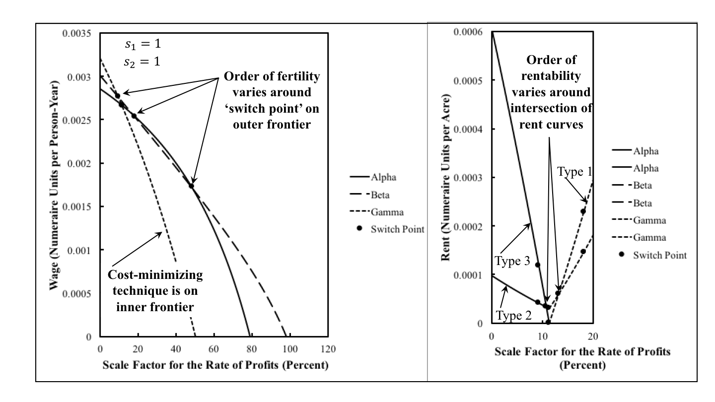
Figure 1: Wage Curves and Rent for an Example of Intensive Rent

1.0 Introduction

This post is one in a series exploring variations of an example from Antonio D'Agata (1983).

This post demonstrates that at least one of my fluke cases can appear in a model of intensive rent by varying a parameter specifying relative markups among sectors. This post is only a start of exploring the parameter space of relative markups in a specific numeric example of intensive rent.

Suppose the rate of profits is given, subject to the constraint that the ratios of the rate of profits in agriculture to that in other industries are as specified. Then the wage can be one of two distinct levels. When the wage is at the lower level, then the rent per acre is higher and vice versa. On the other hand, an increased wage, when it is at the lower level is associated with an increased rate of profits.

2.0 Technology, Requirements for Use, Endowments, and Relative Markups

Table 1 presents coefficients of production in an example from D'Agata (1983). Only one type of land exists, and three processes are known for producing corn on it. The scarcity of land is shown by the possibility of two corn-producing processes being operated side-by-side in the cost-minimizing technique.

Table 1: The Coefficients of Production

Input	Industry
	Iron	Steel	Corn
	I	II	III	IV	V
Labor	1	1	1	11/5	1
Land	0	0	1	1	1
Iron	0	0	1/10	1/10	1/10
Steel	0	0	2/5	1/10	1/10
Corn	1/10	3/5	1/10	3/10	2/5

Following D'Agata, assume that one hundred acres of land are available and that net output consists of 90 tons iron, 60 tons steel, and 19 bushels corn. The net output is also the numeraire. All three commodities must be produced for any composition of net output. Table 2 lists the available techniques. Only Alpha, Delta, and Epsilon are feasible for these requirements for use. Not all land is farmed and only one corn-producing process is operated under Alpha. Two corn-producing processes are operated together under Delta and Epsilon.

Table 2: Techniques

Technique	Processes
Alpha	I, II, III
Beta	I, II, IV
Gamma	I, II, V
Delta	I, II, III, IV
Epsilon	I, II, III, V
Zeta	I, II, IV, V

In the non-competitive case, the relative markups in different industries are taken as given. Let the rates of profits be in proportions of s₁, s₂, and s₃, respectively.

3.0 Prices of Production

Prices of prodution can be defined for each technique. Each process operated in a technique contributes an equation in which the going rate of profits are obtained for that industry. The rate of profits in producing iron is s₁ r. In steel, it is s₂ r, and it is s₃ r in the corn-producing processes. As in past posts, I call r the scale factor for the rate of profits.

For example, the following equations specify prices of production for the Delta technique:

(p₁ a_1,1 + p₂ a_2,1 + p₃ a_3,1)(1 + s₁ r) + w a_0,1 = p₁

(p₁ a_1,2 + p₂ a_2,2 + p₃ a_3,2)(1 + s₂ r) + w a_0,2 = p₂

(p₁ a_1,3 + p₂ a_2,3 + p₃ a_3,3)(1 + s₃ r) + ρ c₃ + w a_0,2 = p₃

(p₁ a_1,4 + p₂ a_2,4 + p₃ a_3,4)(1 + s₃ r) + ρ c₄ + w a_0,3 = p₃

In these equations, p₁, p₂, and p₁ are the prices of iron, steel, and corn. The wage is denoted by w, and ρ denotes rent per acre. The techology provides the coefficients of production in this system of equation. The specification of the numeraire specifies another equation.

90 p₁ + 60 p₂ + 19 p₃ = 1

One degree of freedom remains. I take the the scale factor for the rate of profits as externally given in this post.

In solving the above system, a linear combination of the two equations for corn-producing processes can be taken such that rent drops out. Prices of iron, steel, and corn and the wage can be found first. Then one can obtain rent per acre from either one of the corn-producing processes. Only ranges of the scale factor are considered in which prices, the wage, and rent are non-negative.

4.0 Choice of Technique

A technique is cost-minimizing, at a given scale factor for the rate of profits, if it is feasible and extra profits cannot be obtained by operating any process outside the technique. In evaluating a process to see if extra profits can be obtained by running it, one uses the prices of production determined by the technique and the scale factor for the rate of profits. Extra profits in the processes comprising the technique are zero, neither positive nor negative.

Figure 2: Extra Profits for Alpha Prices

Figure 2 shows that Alpha is cost-minimizing only at the scale factor for the rate of profits. If the scale factor were less than this, extra profits would be gained by combining the last corn-producing process with the first. That is, starting from the Alpha technique, capitalists in agriculture would adopt the Epsilon technique. As demonstrated by the right pane in Figure 3, Epsilon is cost-minimizing for any positive scale factor for the rate of profits up to that at the switch point. Delta is cost-minimizing from a scale factor for the rate of profits where the rate of profits turns positive up to the switch point.

Figure 3: Extra Profits for Delta and Epsilon Prices

Above the switch point, the rate of profits for Alpha is positive up to a certain maximum. In this range, extra profits can be made by operating process IV. The Beta technique would be selected if this process entirely replaced the corn-minimizing technique in Alpha. But Beta is not feasible. On the other hand, processes III and IV are operated side-by-side in the Delta technique. But in this range for the scale factor for the rate of profits, Delta obtains a negative rent. So no cost-minizing technique exists for a scale factor for the rate of profits greater than that at a switch point.

Table 3: Cost-Minimizing Techniques

Lower Bound on r	Upper Bound on r	Techniques
0 percent	11.1 percent	Delta has a negative wage
		Epsilon has a positive wage and positive rent
		Epsilon is uniquely cost-minimizing
11.1 percent	43.9 percent	Delta has a positive wage and positive rent
		Epsilon has a positive wage and positive rent
		Delta is non-uniquely cost-minimizing
		Epsilon is non-uniquely cost-minimizing
43.9 percent	65.5 percent	Delta has negative rent
		Epsilon has a positive wage and negative rent
		Alpha has a positive wage
		No cost-minimizing technique exists

Table 3 summarizes this analysis of the cost-minimizing technique for this fluke case with markup pricing and intensive rent. Before the switch point, the wage frontier consists of both the wages curves for the Delta and Epsilon techniques. The wage frontier does not exist after the switch point. D'Agata's original example, with competitive markets, also illustrates the possibility of a range of the rate of profits with multiple cost-minimizing techniques away from a switch point. And he also notes the possibility of the non-existence of a cost-minimizing technique.

5.0 Conclusion

Fluke cases are associated with qualitative change in the analysis of the choice of technique. Such fluke cases can be brought about by technological improves, that is, changes in coefficients of production. This numerical example illustrates that one of these fluke cases can also be brought about changes in market power between agriculture and industry. In this fluke case, three wage curves intersect at a single switch point.

If agriculture does not have quite as much market power as in the example, a range of the scale factor for the rate of profits exists where both Alpha and Delta are cost-minimizing. For the higher wage, landlords cannot exist since land is not scarce and obtains no rent. This variation in whether or not land is scarce with variations in distribution is not about net output. The level and composition of net output is taken as fixed in the above analysis. The fluke case is associated with the disappear of the range of the rate of profits in which Alpha is cost-minimizing. If agriculture has more market power than in the example, Alpha is never cost-minimizing.

This particular example of markup pricing and intensive rent can be further explored. What other fluke cases exist? What happens if the iron and steel industries do not have the same market power?

Reference

• D'Agata, Antonio. 1983. The existence and unicity of cost-minimizing systems in intensive rent theory. Metroeconomica 35: 147-158'

Franz Fanon On The Need For People And Leaders To Learn

Optimism of the will leads me to hope that, with the misery we endure and cause, someday some people, including leaders of political movements and parties, will gain some wisdom. As I understand it, Frantz Fanon generalized principally from Algeria.

The settler is not simply the man who must be killed. Many members of the mass of colonialists reveal themselves to be much, much nearer to the national struggle than certain sons of the nation. The barriers of blood and race-prejudice are broken down on both sides. In the same way, not every Negro or Moslem is issued automatically a hallmark of genuineness; and the gun or the knife is not inevitably reached for when a settler makes his appearance. Consciousness slowly dawns upon truths that are only partial, limited, and unstable. As we may surmise, all this is very difficult. The task of bringing the people to maturity will be made easier by the thoroughness of the organization and by the high intellectual level of its leaders. The force of intellect increases and becomes more elaborate as the struggle goes on, as the enemy increases his maneuvers and as victories are gained and defeats suffered. The leaders show their power and authority by criticizing mistakes, using every appraisal of past conduct to bring the lesson home, and thus insure fresh conditions for progress. Each local ebb of the tide will be used to review the question from the standpoint of all villages and of all political networks. The rebellion gives proof of its rational basis and expresses its maturity each time that it uses a particular case to advance the people's awareness. In defiance of those inside the movement who tend to think that shades of meaning constitute dangers and drive wedges into the solid block of popular opinion, the leaders stand firm upon those principles that have been sifted out in the national struggle, and in the worldwide struggle of mankind for his freedom. There exists a brutality of thought and a mistrust of subtlety which are typical of revolutions; but there also exists another kind of brutality which is astonishingly like the first and which is typically anti-revolutionary, hazardous, and anarchist. This unmixed and total brutality, if not immediately combated, invariably leads to the defeat of the movement within a few weeks.

The nationalist militant who had fled from the town in disgust at the demagogic and reformist maneuvers of the leaders there, disappointed by political life, discovers in real action a new form of political activity which in no way resembles the old. These politics are the politics of leaders and organizers living inside history who take the lead with their brains and their muscles in the fight for freedom. These politics are national, revolutionary, and social and these new facts which the native will now come to know exist only in action. They are the essence of the fight which explodes the old colonial truths and reveals unexpected facets, which brings out new meanings and pinpoints the contradictions camouflaged by these facts. The people engaged in the struggle who because of it command and know these facts, go forward, freed from colonialism and forewarned of all attempts at mystification, inoculated against all national anthems. Violence alone, violence committed by the people, violence organized and educated by its leaders, makes it possible for the masses to understand social truths and gives the key to them. Without that struggle, without that knowledge of the practice of action, there's nothing but a fancy-dress parade and the blare of the trumpets. There's nothing save a minimum of readaptation, a few reforms at the top, a flag waving: and down there at the bottom an undivided mass, still living in the middle ages, endlessly marking time. -- Frantz Fanon, The Wretched of the Earth, Chapter 2: Spontaneity: its strengths and weaknesses

I think by 'violence' Fanon (and Georges Sorel before him) are talking about organized direct action.

Elsewhere

The First Of A Robert Paul Wolff Series Of Lectures On Marx

• Wolff raises the question of why Marx writes like he does in the first volume of Capital. The rest of Wolff's lectures:
• Lecture 2
• Lecture 3
• Lecture 4
• Lecture 5
• Lecture 6
• Lecture 7
• Seth Ackerman, in Jacobin, on Marxist crisis theory.
• Nathan Robinson pans Thomas Sowell.
• Unlearning Economics disagrees with Sabine Hossenfelder. (Her original video.)

Marx Against A Simple Labor Theory Of Value

Marx distinguishes, at least, between market prices, prices of production, and labor values. For the first volume of Capital, Marx assumes market prices bob around or tend to labor values, not prices of production. I think Marx nowhere says he is assuming the organic composition of capital does not vary among industries. He adopts the labor theory of value in when considering capitalist production as a whole so as to address the question of how owners of capital are able to regularly obtain a profit. He wants this explanation to apply when capitalists are not cheating each other. Nor are they cheating the workers.

I have noted before a few passages in the first volume where Marx demonstrates that he is making a simplification, to be dropped in volume 3. Consider the following:

"If prices actually differ from values, we must, first of all, reduce the former to the latter, in other words, treat the difference as accidental in order that the phenomena may be observed in their purity, and our observations not interfered with by disturbing circumstances that have nothing to do with the process in question. We know, moreover, that this reduction is no mere scientific process. The continual oscillations in prices, their rising and falling, compensate each other, and reduce themselves to an average price, which is their hidden regulator. It forms the guiding star of the merchant or the manufacturer in every undertaking that requires time. He knows that when a long period of time is taken, commodities are sold neither over nor under, but at their average price. If therefore he thought about the matter at all, he would formulate the problem of the formation of capital as follows: How can we account for the origin of capital on the supposition that prices are regulated by the average price, i. e., ultimately by the value of the commodities? I say 'ultimately', because average prices do not directly coincide with the values of commodities, as Adam Smith, Ricardo, and others believe." -- Marx, Capital, volume 1, last footnote in chapter 5.

Marx above distinguishes between what he will come to call prices of production and labor values. Labor values, for Marx, are important for the economy as a whole. But individual prices are attracted by prices of production, not labor values. Or again:

"The calculations given in the text are intended merely as illustrations. We have in fact assumed that price = values. We shall, however, see, in Book III, that even in the case of average prices the assumption cannot be made in this very simple manner." -- Marx, Capital, volume 1,last footnote in chapter 9, section 1

He is explicit above that the calculations are examples, not literally true. But the occassion of this post was when I stumbled across the following:

"The law demonstrated above now, therefore, takes this form: the masses of value and of surplus value produced by different capitals - the value of labour power being given and its degree of exploitation being equal - vary directly as the amounts of the variable constituents of these capitals, i.e., as their constituents transformed into living labour power.

This law clearly contradicts all experience based on appearance. Everyone knows that a cotton spinner, who, reckoning the percentage on the whole of his applied capital, employs much constant and little variable capital, does not, on account of this, pocket less profit or surplus value than a baker, who relatively sets in motion much variable and little constant capital. For the solution of this apparent contradiction, many intermediate terms are as yet wanted, as from the standpoint of elementary algebra many intermediate terms are wanted to understand that 0/0 may represent an actual magnitude. Classical economy, although not formulating the law, holds instinctively to it, because it is a necessary consequence of the general law of value. It tries to rescue the law from collision with contradictory phenomena by a violent abstraction. It will be seen later how the school of Ricardo has come to grief over this stumbling-block. Vulgar economy which, indeed, 'has really learnt nothing', here as everywhere sticks to appearances in opposition to the law which regulates and explains them. In opposition to Spinoza, it believes that 'ignorance is a sufficient reason'." -- Marx, Capital, volume 1, Chapter 9, Rate and mass of surplus value.

I would like to say volume 1, being the only volume of Capital Marx published in his lifetime, should be central in understanding his theory. The above is another demonstration in opposition to this view, at least as far as the analysis of capital goes. In a even larger project, Marx intended to "examine the system of bourgeois economy in the following order: capital, landed property, wage-labour; the State, foreign trade, world market." It is arguable that some of these steps were incorporated into Capital, but he never arrived at the last three.

No where in this post do I address Marx's curious rhetoric. He talks about real illusions, uses Hegelian terminology, and a lot of fierce irony.

As a throwaway comment, let me note one area where I think Marx is weak. Why do the workers consitute a universal class? Why did Marx think the next social revolution would be the last, ending humanity's prehistory? He provides a philosophical derivation of the role of the working class in such early works as Critique of Hegel's Philosophy of Right and The German Ideology. This derivation in tension with the empiricalism that one should build on the materialist theory of history. Since then, we have seen Lenin and Mao look at the role of the peasants in revolutions in less developed areas of the world. Franz Fanon looked at the global south and the revolutions accompanying decolonization. Michael Hardt and Antonio Negri talk about the 'multitude'. You may have noticed that I do not talk much about praxis. But do workers around the world still have a privileged position in hopes for social change?

Jeremy Rudd: "Why I hate economics"

Jeremy Rudd addresses the Cambridge Society for Economic Pluralism

Jeremy Rudd has written:

Mainstream economics is replete with ideas that 'everyone knows' to be true, but that are actually arrant nonsense. For example, 'everyone knows' that:

• aggregate production functions (and aggregate measures of the capital stock) provide a good way to characterize the economy's supply side;
• over a sufficiently long span - specifically, one that allows necessary price adjustments to be made - the economy will return to a state of full market clearing; and
• the theory of household choice provides a solid justification for downward-sloping market demand curves.

None of these propositions has any sort of empirical foundation; moreover, each one turns out to be seriously deficient on theoretical grounds¹. Nevertheless, economists continue to rely on these and similar ideas to organize their thinking about real-world economic phenomena. No doubt one reason why this situation arises is because the economy is a complicated system that is inherently difficult to understand, so propositions like these - even though wrong - are all that saves us from intellectual nihilism. Another, more prosaic reason is Stigler's (1983, p. 541) equally nihilistic observation that 'it takes a theory to beat a theory.'

Is this state of affairs ever harmful or dangerous? One natural source of concern is if dubious but widely held ideas serve as the basis for consequential policy decisions².

¹ For a useful brief against production functions, see Felipe and Fisher (2003); for the case against capital aggregates, see Brown (1980). The idea that the inherent stability of the economy is a concomitant of general-equilibrium theory is difficult to entertain seriously after giving Fisher (1983) close study; see Grandmont (1982) for some related macroeconomic arguments. Finally, Hildenbrand (1994) provides a sobering corrective to first-year demand theory.

² I leave aside the deeper concern that the primary role of mainstream economics in our society is to provide an apologetics for a criminally oppressive, unsustainable, and unjust social order.

The above quote is from a paper about inflations expectations. I wondered how far and on what grounds Rudd thinks this arrant nonsense extends. The talk in the video linked to the top of this post helps answer this question.

Extensive Rent, Absolute Rent, and Markup Pricing

Figure 1: Variation of Technique with Relative Markups

1.0 Introduction

This is a rewrite of a previous post with somewhat 'nicer' values for coefficients of production. I also expand on it with some observations on absolute rent. As far as I know, these posts are the first explicit presentation in the post-Sraffian tradition of a model of the prices of production with extensive rent and markup pricing.

These posts explore the conflict over distribution among workers, capitalists, and landlords. In a model of extensive rent, perturbations of relative market power among industries can create or destroy reswitching of the orders of fertility or of rentability. Extensive rent, called ‘differential rent of the first kind’ by Marx, arises when different types of land are cultivated. The same commodity, 'corn', is produced on each type of land, with a different mixture of labor and material inputs on each. An industrial commodity, 'iron', is produced in the numerical example explored in this article, thereby ensuring that capital consists of heterogeneous products.

2.0 Technology

Table 1 presents the technology for the example. The second column shows the inputs of labor, iron, and corn needed to produce a ton of iron. The remaining three columns to the right are the coefficients of production for processes to produce corn. A unit level of operation of a process in agriculture produces a bushel corn and requires an input of one of three types of land, as shown. Constant returns to scale prevail, although the level of operation of the processes producing corn is limited by the available acreage. This example has the same structure as a previous example, with different numbers.

Table 1: The Coefficients of Production

Input	Industry
	Iron	Corn
	I	II	III	IV
Labor	1 person-yr.	9/10 person-yrs.	6/10 person-yr.	29/50 person-yr.
Type I Land	0	1 acre	0	0
Type II Land	0	0	49/50 acre	0
Type III Land	0	0	0	2/5 acre
Iron	9/20 ton	1/40 ton	3/2000 ton	29/500 ton
Corn	2 bushels	1/10 bushel	9/20 bushel	13/100 bushel

In the three processes for producing corn, process III requires more labor per acre of land than process II, and process IV requires even more. Output per acre of land also increases across these three processes. Process III requires less seed corn per acre than process II, and process IV requires even less. Given these contrasts, processes II, III, and IV cannot be ranked by physical efficiency alone. Iron inputs per acre do not even vary monotonically among processes II, III, and IV, further illustrating the need for prices to rank lands by efficiency.

The given data includes the land available and the requirements for use. These are such that all three type of land must be at least partially farmed. Specifically, 100 acres of each type of land exist, and net output consists of 300 bushels corn. Three hundred bushels of corn is taken as the numeraire. The given data are in principle observable at a single moment in time. Different types of land are distinguished by how corn is grown on them. No need exists to imagine marginal adjustments (Gehrke 2021).

Three techniques, Alpha, Beta, and Gamma, can feasibly satisfy requirements for use. In all three techniques, all four processes are operated. One of the types of land is not fully cultivated in each technique (Table 2). The choice of technique is based on cost-minimization or profit maximization.

Table 2: Techniques of Production

Technique	Land
	Type 1	Type 2	Type 3
Alpha	Partially farmed	Fully farmed	Fully farmed
Beta	Fully farmed	Partially farmed	Fully farmed
Gamma	Fully farmed	Fully farmed	Partially farmed

3.0 Prices of Production

Prices of production are here defined for a given ratio of markups in the industrial and agriculture sectors. The rate of profits in the process producing iron is s₁ r, while the rate of profits in each of the three processes producing corn is s₂ r. I call r the scale factor for the rate of profits. Prices of production satisfy the following system of equations:

(p₁ a_1,1 + p₂ a_2,1)(1 + s₁ r) + w a_0,1 = p₁

(p₁ a_1,2 + p₂ a_2,2)(1 + s₂ r) + ρ₁ c_1,2 + w a_0,2 = p₂

(p₁ a_1,3 + p₂ a_2,3)(1 + s₂ r) + ρ₂ c_2,3 + w a_0,3 = p₂

(p₁ a_1,4 + p₂ a_2,4)(1 + s₂ r) + ρ₃ c_3,4 + w a_0,4 = p₂

I am assuming that wages and rents are paid out of the surplus at the end of the period of production. The relative market power of industry over industry, or vice versa, is expressed by the ratio s₁/s₂. When this ratio is unity, the equations characterize a competitive capitalist economy.

Each of the processes in the technology contributes an equation to the system of equations defining prices of production. The rate of profits is calculated on the value of the capital goods advanced. Rent and wages are paid out of the surplus. Four equations are defined in terms of seven variables, the prices of iron and corn, the rents per acre on each of the three types of land, the wage, and the scale factor for the rate of profits. The coefficients of production and the markups s₁ and s₂ are taken as given.

The following equation specifies that the rent on at least one type of land is zero:

ρ₁ ρ₂ ρ₃ = 0

Specifying the numeraire removes one degree of freedom:

300 p₂ = 1

All rents must be non-negative and one type of land must pay no rent. This is the type of land not fully cultivated. This constraint removes another degree of freedom. The following equation specifies that the rent on at least one type of land is zero:

ρ₁ ρ₂ ρ₃ = 0

This constraint removes another degree of freedom. The system of equations for prices of production has one degree of freedom for this model of markup pricing with extensive rent. This degree of freedom can be expressed as a function showing how the wage decreases with the scale factor for the rate of profits. With the rate of profits somehow specified, the wage, the price of iron, and rent on the scarce land are determined.

4.0 The Choice of Technique: An Example with Competitive Markets

Figure 2 illustrates wage and rent curves when s₁ and s₂ are unity. Markets are competitive, and the scale factor for the rate of profits is merely the rate of profits. The cost-minimizing technique corresponds to the wage curve on the inner frontier.

Consider a rate of profits of zero or just barely positive. Alpha is cost-minimizing. If the requirements for use were small enough that they could be satisfied by only farming Type 3 land, a technique with same wage curve as Gamma would be cost-minimizing. No land would pay rent and the wage would be as shown on the highest wage curve. With somewhat greater requirements for use, Type 2 land would be taken into cultivation, and the wage would be as shown on the wage curve for Beta. Type 3 land would be fully cultivated and pay a rent. Finally, with the originally postulated requirements for use, Type 1 land is cultivated. In the range for the smallest rate of profits, the order of fertility, from most fertile to least fertile land, is Type 3, Type 2, Type 1.

Figure 2: Wage and Rent Curves with Competitive Markets

Alpha is still cost-minimizing for a rate of profits greater than that at the first intersection on the outer frontier for the wage curves, but smaller than that at the switch point on the inner frontier of the wage curves. For a given rate of profits the order of fertility is from the type of land associated with the technique with the highest wage curve downwards. In this range of the rate of profits, the order of fertility is Type 2, Type 3, Type 1.

This is an example of the reswitching of the order of fertility. When Gamma is cost-minimizing, the order of fertility varies from Type 2, Type 1, Type 3 lands to Type 1, Type 2, Type 3 lands and back. The wage curve for the Beta technique is never on the inner frontier, and Beta is never cost-minimizing.

Rent curves are graphed on the right pane in Figure 2. For each switch point for the wage curves, a pair of points, vertically stacked, are shown on the graph of rent curves. For the switch points on the inner frontier of the wage curves, two rent curves intersect at a rent of zero. Type 1 and Type 3 lands pay no rent at this switch point. The switch points for the intersections on the outer frontier of wage curves are not striking on the graph of the rent curves.

The intersections for the rent curves occur at rates of profits different from those for which wage curves intersect. When Alpha is cost-minimizing, the order of rentability varies from Type 3, Type 2, Type 1 to Type 2, Type 3, Type 1. The order of fertility first matches the order of rentability, then deviates from it at a higher rate of profits, then matches again at a still higher rate of profits. Whether or not the orders of fertility and rentability match also varies with the rate of profits in the range where Gamma is cost-minimizing and Type 3 land pays no rent.

Figure 3: Distribution of National Income with Competitive Markets

Given net output and the rate of profits, the levels of operation of each process, the prices of their inputs, and the value of the components of net output are defined. Figure 3 plots total wages, rent, and profits as functions of the rate of profits. Since net output is taken as numeraire, these components add up to unity, whatever the rate of profits. Wages decrease and profits increase with the rate of profits, but rents do not vary monotonically. When Type 1 land is non-scarce, total rents decrease with the rate of profits. When Type 3 land is non-scarce, on the other hand, total rents increase with the rate of profits.

5.0 Perturbing Relative Markups

The non-competitive case can differ qualitatively from the competitive case presented in Section 4. In a non-competitive case, with agriculture having sufficient market power, Beta is sometimes cost-minimizing. This is never so in the competitive case. Throughout the range for the scale factor for the rate of profits in which the Alpha technique is cost-minimizing in this non-competitive case, the orders of efficiency and rentability do not vary. The same is true for the range of the scale factor in which Gamma is cost-minimizing. The opposite is true in the competitive case, and sometimes the order of rentability does not match the order of fertility when Alpha or Gamma are cost-minimizing.

One can construct an overall picture of how these changes come about by analyzing the full range of possible ratios of the markup in industry to the markup in agriculture. The heavy, solid lines in Figure 1, at the top of this post, are switch points on the inner frontier of the wage curves and the maximum scale factor for the rate of profits. The cost-minimizing technique is labeled. The dashed lines are intersections on the outer frontier of the wage curves. The order of fertility varies across dashed lines. Dotted lines are intersections of rent curves. The order of rentability varies across dotted lines. Dashed lines are hard to perceive to the right, when industry has more market power than agriculture.

Figure 4: Enlargement of Variation with Relative Markups

Thin vertical lines partition the axis for the ratio of markups. Each vertical line corresponds to a fluke case. Figure 4 enlarges the left part of the figure, where agriculture has the most market power. For the first fluke case, the rent curves for Type 1 and Type 3 lands, when Beta is cost-minimizing, become tangent at the indicated ratio of markups. The partition between the second and third region is a fluke case where the second intersection for the rent curves for Type 1 and Type 3 lands occurs at the maximum value for the scale factor for the rate of profits. At the ratio for markups for the third fluke case, the wage curves for Beta and Gamma techniques intersect with a wage of zero. The fourth fluke case is a ratio of markups such that all three wage curves intersect at a single switch point. The rents of all three types of land are zero at that switch point. The fifth fluke case, at a partition between Regions 5 and 6, is such that the wage curves for Alpha and Beta intersect at the maximum scale factor for the Gamma technique. The wage curves for the Alpha and Beta techniques are tangent at a switch point for the ratio of markups at the last fluke case.

Table 3 summarizes this numeric example. Variations in the cost-minimizing technique, in the order of fertility, and in the order of rentability with the scale factor for the rate of profits are indicated. In Region 1, agriculture has the most extreme level of market power over industry. The wage curve for Alpha intersects the wage curve for Beta on the inner frontier and then the wage curve for Gamma on the outer frontier. The rent curves do not intersect in the appropriate ranges of the scale factor for the rate of profits. The order of rentability only varies with the cost-minimizing technique.

Table 3: Variations in the Cost-Minimizing Technique

Region	Range	Technique	Order of Fertility	Order of Rentability
1	0 ≤ r ≤ r1	Alpha	Type 3, 2, 1	Type 3, 2, 1
	r1 ≤ r ≤ r2	Beta	Type 3, 1, 2	Type 3, 1, 2
	r2 ≤ r ≤ rmax, β		Type 1, 3, 2
2	0 ≤ r ≤ r1	Alpha	Type 3, 2, 1	Type 3, 2, 1
	r1 ≤ r ≤ r2	Beta	Type 3, 1, 2	Type 3, 1, 2
	r2 ≤ r ≤ r*		Type 1, 3, 2
	r* ≤ r ≤ r**			Type 1, 3, 2
	r** ≤ r ≤ rmax, β			Type 3, 1, 2
3	0 ≤ r ≤ r1	Alpha	Type 3, 2, 1	Type 3, 2, 1
	r1 ≤ r ≤ r2	Beta	Type 3, 1, 2	Type 3, 1, 2
	r2 ≤ r ≤ r*		Type 1, 3, 2
	r* ≤ r ≤ rmax, β			Type 1, 3, 2
4	0 ≤ r ≤ r1	Alpha	Type 3, 2, 1	Type 3, 2, 1
	r1 ≤ r ≤ r2	Beta	Type 3, 1, 2	Type 3, 1, 2
	r2 ≤ r ≤ r*		Type 1, 3, 2
	r* ≤ r ≤ r3			Type 1, 3, 2
	r3 ≤ r ≤ rmax, γ	Gamma	Type 1, 2, 3	Type 1, 2, 3
5	0 ≤ r ≤ r1	Alpha	Type 3, 2, 1	Type 3, 2, 1
	r1 ≤ r ≤ r*		Type 2, 3, 1
	r* ≤ r ≤ r2			Type 2, 3, 1
	r2 ≤ r ≤ r**	Gamma	Type 2, 1, 3	Type 2, 1, 3
	r** ≤ r ≤ r3			Type 1, 2, 3
	r3 ≤ r ≤ rmax, γ		Type 1, 2, 3
6	0 ≤ r ≤ r1	Alpha	Type 3, 2, 1	Type 3, 2, 1
	r1 ≤ r ≤ r*		Type 2, 3, 1
	r* ≤ r ≤ r2			Type 2, 3, 1
	r2 ≤ r ≤ r**	Gamma	Type 2, 1, 3	Type 2, 1, 3
	r** ≤ r ≤ r3			Type 1, 2, 3
	r3 ≤ r ≤ r4		Type 1, 2, 3
	r4 ≤ r ≤ rmax, γ		Type 2, 1, 3
7	0 ≤ r ≤ r1	Alpha	Type 3, 2, 1	Type 3, 2, 1
	r1 ≤ r ≤ r*		Type 2, 3, 1
	r* ≤ r ≤ r2			Type 2, 3, 1
	r2 ≤ r ≤ r**	Gamma	Type 2, 1, 3	Type 2, 1, 3
	r** ≤ r ≤ rmax, γ			Type 1, 2, 3

Region 2, and the fluke cases bounding it, illustrates that a persistent change in the relative market power among industries can bring about the reswitching of the order of rentability. The rent curves for Type 1 and Type 3 land intersect twice in the range of the scale factor of profits in which Beta is cost-minimizing. The rent curves for both types of land are increasing functions of the scale factor in this range.

The rent curve for Type 3 land becomes downward-sloping in Region 3. It is not always monotone. The order of rentability at the highest range of the scale factor for the rate of profits in Region 2 has disappeared in Region 3. With some thought, one can see how the variations between regions in the ranges of the scale factor for the cost-minimizing technique, the order of fertility, and the order of rentability relate to the fluke cases dividing these regions. The range of the scale factor in which Beta is cost-minimizing has disappeared in Region 5, after the switch point at which all three wage curves intersect. Switch points between Alpha and Beta and between Beta and Gamma are thenchforth on the outer wage frontier and are the occasion of a change in the order of fertility. Region 6 is an example of the reswitching of the order of fertility, and is illustrated in Section 4 with the competitive case. In Region 7, the last in the table, the order of fertility does not vary when Gamma is cost-minimizing.

6.0 Conclusion

The numerical example illustrates complications that can arise in the conflict over the distribution of the surplus among workers, capitalists in various industries, and owners of types of land. I take the coefficients of production as frozen in considering this conflict. That is, I do not consider the conflict over the length of the working day, the intensity with which workers work, the care they must take to prevent waste, the right to urinate on the job, and so on. Nor do I consider some conflicts between capitalists and landlords, outside of distribution. For example, landlords would like leases as short as possible so as to be able to raise rents for more-or-less permanent improvements brought about by the capitalists, while the capitalists would like longer rents to prevent this outcome.

The model illustrated above is one in which relative markups are given. It demonstrates that in the competitive case, the order of fertility of lands can vary with the rate of profits, where the rate of profits is taken as given from outside the model. The order of fertility can vary both with and without the cost-minimizing technique varying. The order of lands from high rent to low rent lands also varies, in general, with the rate of profits. One may find that ownership of one type of asset provides greater returns than another, even though the latter asset is more efficient at the going rate of profits.

Persistent differences in markups among industries does not alter these conclusions, but does provide the possibility of qualitative and quantitative variation in details. In the example, if agriculture has sufficient market power over industry, the example no longer exhibits a reswitching of the order of fertility. A range of the scale factor for the rate of profits emerges in which type 2 land no longer obtains a rent. An even further increase in the market power of agriculture can lead to the appearance and the disappearance of the reswitching of the order of rentability

No simple picture emerges from this analysis. The workers can only obtain a larger share of the surplus product if the capitalists get less. Whether or not the landlords are able to obtain a larger share with either an increased rate of profits or increased market power for some sectors varies

Ludwig Von Mises Being Stupid

Are those who obtain more income better in some way, perhaps more intelligent than others? Are they luckier? According to Ludwig Von Mises, they are superior in intelligence:

"The entrepreneur is the agency that prevents the persistence of a state of production unsuitable to fill the most urgent wants of the consumers in the cheapest way. All people are anxious for the best possible satisfaction of their wants and are in this sense striving after the highest profit they can reap. The mentality of the promoters, speculators, and entrepreneurs is not different from that of their fellow men. They are merely superior to the masses in mental power and energy. They are the leaders on the way toward material progress. They are the first to understand that there is a discrepancy between what is done and what could be done. They guess what the consumers would like to have and are intent upon providing them with these things. In the pursuit of such plans they bid higher prices for some factors of production and lower the prices of other factors of production by restricting their demand for them. In supplying the market with those consumers' goods in the sale of which the highest profits can be earned, they create a tendency toward a fall in their prices. In restricting the output of those consumers' goods the production of which does not offer chances for reaping profit, they bring about a tendency toward a rise in their prices. All these transformations go on ceaselessly and could stop only if the unrealizable conditions of the evenly rotating economy and of static equilibrium were to be attained." -- Von Mises, Human Action, Chapter XVI, Section 3.

You can see why he is popular among plutocrats. His confusion (not demonstrated in this post) about how capitalist economies can work is a feature, not a bug.

Some Notes On Marx On Rent

Marx writes about rent extensively in Part II of Theories of Surplus Value and in volume 3 of Capital. I read Theories of Surplus Value decades ago. I have been trying to read the chapters of volume 3 on rent, that is, chapters 37 to 47.

In general, these chapters do not use Hegelian terminology, but are just a matter of mathematical economics. Marx conflates analyses I would keep separate. Maybe this is a matter of a dynamic analysis set in historical time. I suppose I do not have standing to complain about everything being argued through numerical examples.

In Chapter 37, Marx clarifies that he is discussing ground rent on unimproved land or land with permanent improvements. Capitalist farmers are assumed, along with landed property. He talks about the incentives to tenants not to make improvements. Once a lease runs out, improvements will allow the landlord to raise rents. If the improvements are permanent, these improvements will henceforth enter into ground rents. Marx notes the accounting where the price of land is equal to the discounted value of yearly rents. Even so, the portion of surplus value paid out in rent should not be confused with interest.

Table 1: My Preferred Terminology and Marx's

My Technical Term	Marx's Technical Term
Extensive rent	Differential rent I
Intensive rent	Differential rent II
?	Absolute rent
External intensive rent	?

Chapter 38 starts the analysis of differential rent of the first kind, and Chapter 39 has numeric examples in tables. Marx discusses the case of waterfalls providing power to a factory. Those capitalists without access to the waterfalls, I guess, use steam power. He combines an analysis of physical fertility with nearness to markets. Marx says the most fertile land is not cultivated first. Improvements in transportation can change the ranking of lands. I like the example of the Erie Canal. More than one kind of agricultural product can be produced, but one is dominant in Marx's analysis. Anyways, he considers different arbitrary orders in which lands may be cultivated when discussing extensive rent. Also he considers cases where more of a type of land is discovered; supplies of land are not fixed in the very long run. Prices of production prevail. Capital investments are in monetary terms, despite Marx having shown in earlier chapters that prices of production of, say, seed, fertilizers, ploughs may vary with distribution.

Marx has something like a long-run demand curve for consumer goods:

The ... assumption is that total demand keeps pace with the increase in the total product. First, one need not imagine such an increase coming about abruptly, but rather gradually... Secondly, it is not true that the consumption of necessities of life does not increase as they become cheaper. The abolition of the Corn Laws in England proved the reverse to be the case (F. Newman, Lectures on Political Economy, London, 1851, p.158. — Ed.); the opposite view stems solely from the fact that large and sudden differences in harvests, which are mere results of weather, bring about at one time an extraordinary fall, at another an extraordinary rise, in grain prices. While in such a case the sudden and short-lived reduction in price does not have time to exert its full effect upon the extension of consumption, the opposite is true when a reduction arises from the lowering of the regulating price of production itself, i.e., is of a long-term nature. Thirdly, a part of the grain may be consumed in the form of brandy or beer; and the increasing consumption of both of these items is by no means confined within narrow limits. Fourthly, the matter depends in part upon the increase in population and in part on the fact that the country may be grain-exporting, as England still was long after the middle of the 18th century, so that the demand is not solely regulated within the confines of national consumption. Finally, the increase and price reduction in wheat production may result in making wheat, instead of rye or oats, the principal article of consumption for the masses, so that the demand for it may grow if only for this reason, just as the opposite may take place when production decreases and prices rise. -- Karl Marx, Capital, volume 3, Chapter 39.

Chapter 40 is the start of Marx's discussion of intensive rent, or differential rent of the second kind. He does not discuss it separately from differential rent, but adds it to his analysis. Intensive rent involves the returns to capital, in monetary units, when added to land of a given type. Marx does not treat in agriculture in a complete system. The approach I take to intensive rent is quite different. I am not sure I could always justify Marx's examples with a consistent system of equations, where the number of price and rent variables matches the number of processes, and the wage and the rate of profit frontier provides one degree of freedom. I allow for non-existence and non-uniqueness in these models.

With Marx's approach, he must consider in his numeric examples the possibility of the discovery of any type of land, changes in technology on any type, and the results of additional does of 'capital' on any type of land. He breaks these possibilities into three overarching subcases: A constant price of production of the dominant agriculture product, a falling price of production, and a rising price of production. These cases are discussed in Chapters 41, 42, and 43, respectively. Marx has subcases, in which an additional dose of capital has constant, decreasing, or rising productivity. Which land is on the margin can change. To tell the truth, I did not pay much attention to the details. In Chapter 42, Engels says an error exists in the tables that does not influence the conclusions.

I will update this post when I read further. I am interested if Marx justifies the existence of no cultivated land with no rent by the theory of intensive rent. And where does absolute rent come from?

Extensive Rent and Markup Pricing In A Complicated Example

Figure 1: Variation of Technique with Relative Markups

"That 'diminishing returns' was not an essential element in the surplus-based theory emerged in Marx's criticisms of Ricardo. Sraffa (1960), in his short chapter on land, the implications of which have yet to be developed, shows how the classical view of rents need not necessarily rest on the conception of 'the law of diminishing returns' or need not suggest necessarily any functional relationship between output and cost, or even presume a unique rank ordering of lands according to productivity. In fact, correcting the classical writers, her shows that differential rents as well as the 'no-rent' land depend upon the rate of profit (or wages)." -- Krishna Bharadwaj (1984) Piero Sraffa: A Tribute Economic and Political Weekly 19 (30-1): 1236-1235.

1.0 Introduction

This example illustrates how the struggle over distribution can be complicated. I start with a fluke case, in which three wage curves intersect at a switch point for a model of competitive capitalism with wage labor and extensive rent.

I assume markup pricing, with a stable ratio of the rate in profits in industry to the rate of profits in agriculture. For each such ratio, consider how the choice of the cost-minimizing technique varies with an exogeneous rate of profits. The wage varies, but so do rents per acre, including even which lands pay rent and which do not, because they are not scarce.

This post demonstrates that the introduction of markup pricing into a model of extensive can result in the reswitching of the order of fertility and the reswitching of the order of rentability.

I think I have demonstrated that one can conduct more research in price theory.

2.0 Technology

Table 1 presents the technology for the example. The second column shows the inputs of labor, iron, and corn needed to produce a ton of iron. The remaining three columns to the right are the coefficients of production for processes to produce corn. A unit level of operation of a process in agriculture produces a bushel corn and requires an input of one of three types of land, as shown. Constant returns to scale prevail, although the level of operation of the processes producing corn is limited by the available acreage. This example has the same structure as a previous example, with different numbers.

Table 1: The Coefficients of Production

Input	Industry
	Iron	Corn
	I	II	III	IV
Labor	1 person-yr.	0.89965 person-yrs.	0.60518 person-yr.	0.58085 person-yr.
Type I Land	0	1 acre	0	0
Type II Land	0	0	0.98020 acre	0
Type III Land	0	0	0	0.38724 acre
Iron	9/20 ton	1/40 ton	0.0014882 ton	0.058085 ton
Corn	2 bushels	1/10 bushel	0.45438 bushel	0.12908 bushel

The given data also include the land available and the requirements for use. These are such that all three type of land must be at least partially farmed. Specifically, 100 acres of each type of land exist, and net output consists of 300 bushels corn. Three hundred bushels of corn is taken as the numeriare.

Three techniques, Alpha, Beta, and Gamma, can feasibly satisfy requirements for use. In all three techniques, all four processes are operated. One of the types of land is not fully cultivated in each technique. Table 2 displays which type of land is only partially cultivated in each technique. The choice of technique is based on cost-minimization or profit maximization.

Table 2: Techniques of Production

Technique	Land
	Type 1	Type 2	Type 3
Alpha	Partially farmed	Fully farmed	Fully farmed
Beta	Fully farmed	Partially farmed	Fully farmed
Gamma	Fully farmed	Fully farmed	Partially farmed

2.0 Prices of Production

Prices of production are here defined for a given ratio of markups in the industrial and agriculture sectors. The rate of profits in the process producing iron is s₁ r, while the rate of profits in each of the three processes producing corn is s₂ r. I call r the scale factor for the rate of profits.

Each of the processes in the technology contributes an equation to the system of equations defining prices of production. The rate of profits is calculated on the value of the capital goods advanced. Rent and wages are paid out of the surplus. Four equations are defined in terms of seven variables, the prices of iron and corn, the rents per acre on each of the three types of land, the wage, and the scale factor for the rate of profits. The coefficients of production and the markups s₁ and s₂ are taken as given.

Specifying the numeraire removes one degree of freedom. All rents must be non-negative and one type of land must pay no rent. This is the type of land not fully cultivated. This constraint removes another degree of freedom. The system of equations for prices of production has one degree of freedom for this model of markup pricing with extensive rent. This degree of freedom can be expressed as a function showing how the wage decreases with the scale factor for the rate of profits. With the rate of profits somehow specified, the wage, the price of iron, and rent on the scarce land are determined.

3.0 The Choice of Technique: An Example with Agriculture Having Market Power

Figure 2 illustrates wage curves for the specified markups. Since the ratio s₁/s₂ is less than unity, this is a case in which agriculture has more market power than industry. For a given scale factor for the rate of profits, the order of fertility is from the type of land associated with the technique with the highest wage curve downwards. The cost minimizing technique corresponds to the wage curve on the inner frontier.

Figure 2: Wage Curves with Agriculture Having Market Power

Consider a small scale factor for the rate of profits is such that Alpha is cost-minimizing. If the requirements for use were small enough that they could be satisfied by only farming Type 3 land, Gamma would be cost-minimizing. No land would pay rent and the wage would be as shown on the highest wage curve. With somewhat greater requirements for use, Type 2 land would be taken into cultivation, and the wage would be as shown on the wage curve for Beta. Type 3 land would be fully cultivated and pay a rent. Finally, with the originally postulated requirements for use, Type 1 land is cultivated. In the range for the smallest scale factor for the rate of profits, the order of fertility, from most fertile to least fertile land, is Type 3, Type 2, Type 1.

When Beta is cost-minizing, the order of fertility is Type 3, Type 1, and Type 2 land or Type 1, Type 3, Type 2 land, depending on whether the scale factor for the rate of profits is less than or greater then the scale factor for the rate of profits at the switch point on the outer frontier. For a higher range of the scale factor for the rate of profits, Gamma is cost minimizing, and the order of fertility is Type 1, Type 2, and Type 3 lands.

Figure 3 graphs the rent curves for the specified markups. For each switch point for the wage curves, a pair of points, vertically stacked are shown on the graphs. For the switch points on the inner frontier of the wage curves, two rent curves intersect at a rent of zero. For the first such switch point, Type 2 and Type 1 land pay no rent at the switch point. For the switch point between the Beta and Gamma techniques, Type 3 and Type 2 lands pay no rent at the switch point.

Figure 3: Rent Curves with Agriculture Having Market Power

The switch point for the intersection on the outer frontier between the Alpha and Gamma wage curves is not striking on the graph of the rent curves. One sees one point on one rent curve for the Beta technique above the other.

The intersection for the two rent curves for the Beta technique occurs at a different scale factor for the rate of profits. It is not a scale factor for the rate of profits for which two wage curves intersect. When Beta is cost minimizing, the order of rentability is Type 3, Type 1, Type 2 for scale factors for the rate of profits less than the scale factor at which the rent curves intersect. For greater scale factors, the order of rentability is Type 1, Type 3, Type 2 when Beta is cost-minimizing.

This example demonstrates that the cost-minimizing technique depends on the scale factor for the rate of profits. The order of fertility of types of lands is not uniquely determined by the cost-minimizing technique. Neither is the order of rentability. And these orders do not need to match. One type of land can obtain more rent per acre than another, even when it is less fertile at the given ratio of markups and scale factor for the rate of profits.

4.0 The Choice of Technique: An Example with Industry Having Market Power

Figure 4 presents another graph of wage curves. Here the ratio of markups, s₁/s₂, exceeds unity. Industry has more market power than agriculture. The wage curve for the Beta technique is never on the inner frontier, and Beta is never cost-minimizing. This is an example of the reswitching of the order of fertility. When Gamma is cost-minimizing, the order of fertility varies from Type 2, Type 1, Type 3 lands to Type 1, Type 2, Type 3 lands and back.

Figure 4: Wage Curves with Industry Having Market Power

Figure 5 shows the rent curves for the given markups. Here the order of rentability varies both when the Alpha technique is cost-minimizing amd when the Gamma technique is cost-minimizing.

Figure 5: Rent Curves with Industry Having Market Power

5.0 Perturbing Relative Markups

Figure 1, at the top of this post is an attempt to present a synthetic picture of the example. The heavy, solid lines are switch points on the inner frontier of the wage curves and the maximum scale factor for the rate of profits. The cost minimizing technique is labeled. The dashed lines are intersections on the outer frontier of the wage curves. The order of fertility varies across dashed lines. Dotted lines are intersections of rent curves. The order of rentability varies across dotted lines. Dashed and dotted lines are hard to perceive to the right, when industry has more market power than agriculture.

Thin vertical lines parition the ratio of markups. Each vertical line corresponds to a fluke case. Section 3 is a point in region 4. Section 4 is a point in region 6. Figure 6 enlarges the left of the figure, where agriculture has the most market power. For the first fluke case, the rent curves for Type 1 and Type 3 lands, when Beta is cost-minimizing, become tangent at the indicated ratio of markups. The partition between the second and third case is a fluke care where the second intersection for the rent curves for Type 1 and Type 3 lands occurs at the maximum value for the scale factor for the rate of profits. The second region, and the fluke cases bounding it, illustrates that a persistent change in the relative market power among industries can bring about the reswitching of the order of rentability.

Figure 6: Enlargement of Variation with Relative Markups

In some sense, the ordinate in Figures 1 and 6 should not have units. I drew the graphs by varying s₁, while keeping s₂ constant at unity. But one could double both markups, while cutting the scale factor for the rate of profits in half. The graphs would be unchanged.

Anyways, Table 3 summarizes this numeric example. Variations in the cost-minimizing technique, in the order of fertility, and in the order of rentability with the scale factor for the rate of profits are indicated.

Table 3: Variations in the Cost-Minimizing Technique

Region	Range	Technique	Order of Fertility	Order of Rentability
1	0 ≤ r ≤ r1	Alpha	Type 3, 2, 1	Type 3, 2, 1
	r1 ≤ r ≤ r2	Beta	Type 3, 1, 2	Type 3, 1, 2
	r2 ≤ r ≤ rmax, β		Type 1, 3, 2
2	0 ≤ r ≤ r1	Alpha	Type 3, 2, 1	Type 3, 2, 1
	r1 ≤ r ≤ r2	Beta	Type 3, 1, 2	Type 3, 1, 2
	r2 ≤ r ≤ r*		Type 1, 3, 2
	r* ≤ r ≤ r**			Type 1, 3, 2
	r** ≤ r ≤ rmax, β			Type 3, 1, 2
3	0 ≤ r ≤ r1	Alpha	Type 3, 2, 1	Type 3, 2, 1
	r1 ≤ r ≤ r2	Beta	Type 3, 1, 2	Type 3, 1, 2
	r2 ≤ r ≤ r*		Type 1, 3, 2
	r* ≤ r ≤ rmax, β			Type 1, 3, 2
4	0 ≤ r ≤ r1	Alpha	Type 3, 2, 1	Type 3, 2, 1
	r1 ≤ r ≤ r2	Beta	Type 3, 1, 2	Type 3, 1, 2
	r2 ≤ r ≤ r*		Type 1, 3, 2
	r* ≤ r ≤ r3			Type 1, 3, 2
	r3 ≤ r ≤ rmax, γ	Gamma	Type 1, 2, 3	Type 1, 2, 3
5	0 ≤ r ≤ r1	Alpha	Type 3, 2, 1	Type 3, 2, 1
	r1 ≤ r ≤ r*		Type 2, 3, 1
	r* ≤ r ≤ r2			Type 2, 3, 1
	r2 ≤ r ≤ r**	Gamma	Type 2, 1, 3	Type 2, 1, 3
	r** ≤ r ≤ r3			Type 1, 2, 3
	r3 ≤ r ≤ rmax, γ		Type 1, 2, 3
6	0 ≤ r ≤ r1	Alpha	Type 3, 2, 1	Type 3, 2, 1
	r1 ≤ r ≤ r*		Type 2, 3, 1
	r* ≤ r ≤ r2			Type 2, 3, 1
	r2 ≤ r ≤ r**	Gamma	Type 2, 1, 3	Type 2, 1, 3
	r** ≤ r ≤ r3			Type 1, 2, 3
	r3 ≤ r ≤ r4		Type 1, 2, 3
	r4 ≤ r ≤ rmax, γ		Type 2, 1, 3
7	0 ≤ r ≤ r1	Alpha	Type 3, 2, 1	Type 3, 2, 1
	r1 ≤ r ≤ r*		Type 2, 3, 1
	r* ≤ r ≤ r2			Type 2, 3, 1
	r2 ≤ r ≤ r**	Gamma	Type 2, 1, 3	Type 2, 1, 3
	r** ≤ r ≤ rmax, γ			Type 1, 2, 3

6.0 Conclusion

The numerical example illustrations complications that can arise in the conflict over the distribution of the surplus among workers, capitalists in various industries, and owners of types of land. I take the coefficients of production as frozen in considering this conflict. That is, I do not consider the conflict over the length of the work day, the intensity with which workers work, the care they must take to prevent waste, the right to urinate on the job, and so on. It is hard to summarize the example. For example, for middling values of the scale factor for the rate of profits, owners of Type 2 land receive no rent if agriculture has somewhat more market power than industry. This possibility disappears when industry has more market power than agriculture. Anyways, this is another example in which obtaining a higher rent per acre can be connected with owning a less productive asset.

The coefficients of production in Table 1 are only approximate. My next step is to pick somewhat 'nicer' fractions' where the fluke three-technique switch point need not occur in the competitive special case.

Marginalism As A Distortion Of Classical Rent Theory

I want to note some instances in the literature that argue that one strain in the marginal revolution was an extension of (a misunderstanding of) the theory of intensive rent in classical political economy to all factors of production, particularly capital. This this is not of only historical interest. It suggests that another approach, that of classical political economy, to value and distribution exists. Furthermore, a treatment of intensive rent exists that is opposed to marginalism, in some sense.

The classical theory of rent first became widely known through pamphlets published in February 1815 by Thomas Robert Malthus, David Ricardo, Robert Torrens, and Edward West. James Anderson was an eighteenth century predecessor. Was Karl Marx to first point out that Anderson was overlooked? I have previously provided a taxonomy of some kinds of rent. Pasinetti (2015) has an interesting essay on these pamphlets. He argues Ricardo's was most comprehensive.

Krishna Bharadwaj has an article in which she writes about Marshall's reading of J. S. Mill:

"It is in the third class of commodities, marked by the coexistence of 'several costs of production' and by costs which vary with changes in supply, that provided the basis for the later marginalist conception of a supply function. The law of value in their case is stated by [J. S.] Mill thus: The value is determined by the cost of that portion of the supply which is produced and brought to markt at the greatest expense. (Mill, 1871 [1929], p. 471). To so-called 'law of diminishing returns' was to interest Jevons⁹ and Marshall and to play a significant role in the analytical development of marginalism, through its generalization to situations other than that of explaining rent: 'The law of diminishing marginal utility' was to be its counterpart in the theory of consumption, while it led to a more general notion of diminishing returns to a variable factor in the theory of production (see Bharadwaj, 1978). The Early Writings of Marshall reveal his great interest in the rent doctrine; as he himself remarked, 'improvements in cultivation decided me to adopt curves as an engine' (Marshall, 1975, I, pp. 40-1, p. 41, n. 12). In this third law of value, the functional link between costs and scale of output was clearly evident and provided the ground for a generalized 'supply function'.

⁹ Jevons wrote in the Preface to the first edition of his Theory of Political Economy (included in the fourth edition): 'There are many portions of Economical doctrine which appear to me as scientific in form as they are consonant with facts. I would especially mention the Theories of Population and Rent, the latter a theory of distinctly mathematical character, which seems to give a clue to the correct mode of treating the whole science (Jevons, 1911, p. vi, italics added)." -- Krishna Bharadwaj (1978).

Gehrke (2019) reports on some presentations at the Nationalökonomische Gesellschaft (NOeG), an interwar Vienna circle (not that one). Apparently, Oskar Morgenstern induced them to discuss Sraffa's 1925 article. Karl Menger, the mathematician son of the economist Carl Menger, was inspired by this and a conversation in which Ludwig Von Mises claimed that the law of diminishing returns could be proven. Karl Menger looked at the literature, and found it full of mistakes. The law of diminishing marginal returns could not be validly deduced from the assumptions that marginalist economists made:

"Yesterday ... Menger gave a brilliant paper on the law of dimishing returns. It was an exemplary performance for showing the need for exact reasoning in economics. interestingly, Haberler completely failed in the discussion; I very much noticed this. Of all these exact things he still does not understand the essence. Mises uttered pure nonsense." -- Oskar Morgenstern (31 December 1935, as quoted by Gehrke).

Some decades later Ronald Shepard introduced some arbitrary assumptions 'which are contrived to obtain the result'. Apparently, textbook presentations of increasing supply curves in partial equilibrium analysis of individual markets for consumer goods are still quite confused.

References

• Krishna Bharadwaj. 1978. The subversion of classical analysis: Alfred Marshall's early writings on value. Cambridge Journal of Economics 2(3): 253-271. (Reprined in Krishna Bharadwaj. 1989. Themes in value and distribution. Unwin Hyman)
• Christian Gehrke. 2019. The outstanding NOeG presentations: Morgenstern, Viner, and Menger on the laws of costs and returns. Empirica
• Christian Gehrke. 2021. Differences, switches and 'consistently side by side': Krishna Bharadwaj and the Sraffian critique of economic theory. Indian Economic Journal I-22.
• Luigi L. Pasinetti. 2015. On the origin of the theory of rent in economics. In Resources, Production and Structural Dynamics (ed. by Mauro L. Baranzini, Claudi Rotondi and Roberto Scazzieri). Cambridge University Press.
• Beth Stratford. 2023. Rival definitions of economic rent: historical origins and normative implications. New Political Economy 28(3): 347-362.