This part begins the exposition of the model introduced in the previous part. The exposition is organized into seven subsections in two parts. The first part, consisting of four subsections, describes the corporate sector. The two subsections at the beginning of the second part describe households and financial institutions. The last subsections describes some limitations on parameters that are necessary for the existence of a steady-state growth path in the model.
2.1 Some Accounting Identities
The corporations in this model economy, produce two commodities, steel and corn. Steel can be combined with labor to produce either more steel or corn. Corn is the consumption good. Steel is totally used up in the yearly production processes in the model. Thus, the output of the economy consists of steel to replace the steel used up in production, additional steel to support growth, and corn for consumption.
Let X represent tons steel used in a production cycle, and let p represent the price of steel. The value of capital, K, is given by Equation 1:
Let g be the steady-state rate of growth. Steel output, corn output, the employed labor force, and the value of capital all grow at this rate along a steady-state growth path. Thus, net investment, I, is related to the value of capital by Equation 2:(1)

Equation 3 relates accounting profits, P, to the value of capital:(2)

Equation 3 is a relationship characterizing the return to industrial capital. The returns to industrial capital and to financial instruments are distinguished in this model. It is convenient to follow tradition and refer to r as the rate of profits.(3)
Let w be the wage, and let N be the number of employed person-years. Total wages, W, are then given by Equation 4:
There is no government and no foreign trade in this model. Net income, Y, is paid out in the form of wages and profits:(4)
Equations 1 through 5 are basic identities in this model.(5)

2.2 Finance and the Rate of Profits
The rate of growth is not determined within this model. It is the result of decisions by corporate managers, and it depends on their optimism or pessimism. In short, the rate of growth depends on the "animal spirits" of the corporate managers.
Investment has two sources of finance in the model, retained earnings and the issuing of new stock. Households purchase new stock in the model. Earnings that are not retained are paid out as dividends to stock owners. Let sc be the proportion of profits retained. Let f be the proportion of net investment financed by additional stock. Equation 6 follows:
Some algebraic manipulation yields Equation 7:(6)

One obtains Equation 8 from Equations 2, 3, and 7:(7)

Notice that all the parameters on the right-hand side of Equation 8 are controlled by corporate managers. Thus, the rate of profits on a steady-state growth path is the result of corporate decisions about the rate of growth and the financing of investment.(8)
2.3 Production
Production occurs in the corporate sector. Firms producing steel face the technology defined by the production function in Equation 9:
where a01 is the number of person years labor hired per ton steel produced, and a11 is the number of tons steel used as input per ton steel produced. The technology for producing corn is defined by the production function in Equation 10:(9)

where a02 is the number of person years labor hired per bushel corn produced, and a12 is the number of tons steel used as input per bushel corn produced.(10)
Production functions are assumed to exhibit Constant Returns to Scale and diminishing marginal returns. The inputs of steel are purchased at the start of the year, and the outputs of steel and corn become available at the end of the year. The corporations hire labor for use throughout the year and pay wages at the end of the year.
2.3.1 Price Equations
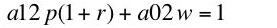
The same rate of profits is earned in each industry along a steady-state growth path:
(11)
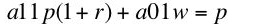
Notice that corn is the numeraire in Equations 11 and 12, and relative prices are constant over time.(12)
Given the coefficients of production, one can solve Equations 11 and 12 for the wage and the price of steel as a function of the rate of profits. Equation 13 gives the wage-rate of profits curve for the technique defined by a choice of the coefficients of production:
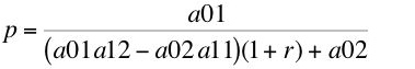
Equation 14 specifies the price of steel, given coefficients of production and the rate of profits:(13)

(14)
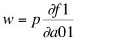
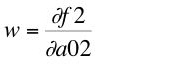
The choice of technique can be analyzed by appending marginal productivity equations to either the system of equations given by Equations 11 and 12 or by Equations 13 and 14. Marginal conditions follow from assuming that competitive firms minimize cost, given technology. Alternatively, one can assume that competitive firms maximize economic profits. Equation 15 shows that the wage is equal to the value of the marginal product of labor in producing steel:
The wage is also equal to the value of the marginal product of labor in producing corn:(15)
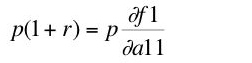
The price of steel, discounted to the end of the year when output becomes available, is equal to the value of the marginal product of steel used in producing steel:(16)
Similarly, the discounted price of steel is equal to the value of the marginal product of steel in producing corn:(17)
(18)

This analysis of the price equations shows that, given the rate of profits, coefficients of production, the wage, and prices of commodities are determined by cost-minimization. Notice no equation exists equating the marginal product of the value of capital, K, and the rate of profits. Marginal productivity conditions are part of the determination of the choice of technique. They do not determine distribution.
2.3.2 Quantity Equations
By assumption, X tons of steel and N person-years of labor are used as inputs in production in a single year. Since the rate of growth is g, (1 + g)X tons of steel are produced and available at the end of the year. Let c be the amount of corn produced per person-year. So c N is the amount of corn produced and available at the end of the year. Equation 19 equates the steel used as input to the sum of the steel inputs in the steel and corn industries:
Equation 20 equates the labor used as input to the sum of the labor inputs in the steel and corn industries:(19)

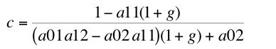
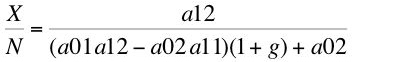
One can solve Equations 19 and 20 for c and X/N as functions of the rate of growth and the coefficients of production. Equation 21 shows the trade-off between per-capita consumption and the rate of growth:(20)

Notice this trade-off is of the same form as the wage-rate of profits curve (Equation 13). Steel per worker is given by Equation 22:(21)
2.4 A Graphical Depiction of Elements of the Corporate Sector(22)
This completes the analysis of the corporate sector. I have shown how, in this model, the rate of profit, the wage, prices, coefficients of production, and quantities produced per worker are determined. Figure 1 summarizes some of this discussion. The blue line in the fourth quandrant plots (the reflection of) Equation 8. In steady state growth, corporate managers have chosen the rate of growth, shown as g* on the abscissa. The corresponding steady state rate of profits, r*, is plotted downward on the ordinate. The graph shows this rate of profits reflected by the 45 degree line back onto the abscissa. The wage-rate of profits curves (Equation 13) for each technique are plotted in the first quadrant. Figure 1 shows two, while the marginal productivity relationships are applicable when an uncountable infinity of such curves exist. The coefficients of production for the chosen technique correspond to the highest wage-rate of profits curve for the rate of profits r*. The corresponding wage, w*, along a steady state growth path is plotted on the ordinate. Likewise, consumption per person-year is plotted on the ordinate by projecting the steady state rate of growth upward to the wage-rate of profits curve for the chosen technique.
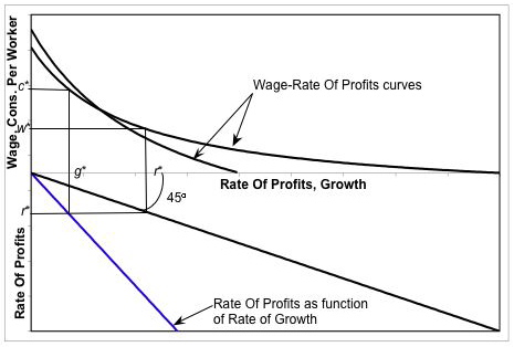 |
| Figure 1: Some Variables Dependent on the Rate of Growth |


2 comments:
Is 8 supposed to be an equilibrium condition or a theory of causation? If the former, it's hard to see how you get "Thus, the rate of profits on a steady-state growth path is the result of corporate decisions about the rate of growth and the financing of investment." If the latter, then your model is wildly different from the real world where managers are constantly coping with the fact that their rate of profit is influenced by countless variables beyond their control.
Both ... and. The concluding post in the series mentions some authors whose work in the theory of the firm is abstracted here.
Post a Comment