Steve Keen: Economists Are "Insufficiently Numerate"

"Curiously, though economists like to intimidate other social scientists with the mathematical rigor of their discipline, most economists do not have this level of mathematical education...

...One example of this is the way economists have reacted to 'chaos theory'... Most economists think that chaos theory has had little or no impact - which is generally true in economics, but not at all true in most other sciences. This is partially because, to understand chaos theory, you have to understand an area of mathematics known as 'ordinary differential equations.' Yet this topic is taught in very few courses on mathematical economics - and where it is taught, it is not covered in sufficient depth. Students may learn some of the basic techniques for handling what are known as 'second-order linear differential equations,' but chaos and complexity begin to manifest themselves only in 'third order nonlinear differential equations.' Steve Keen (2011). Debunking Economics: The Naked Emperor Dethroned?, Revised and expanded ed. Zed Books, p. 31

The above quotes are also in the first edition. Before commenting on this passage, I want to re-iterate my previously expressed belief that some economists, including some mainstream economists, understand differential and difference equations.

I misremembered this comment as being overstated for polemical purposes. But, in context, I think it is clear to those who know the mathematics.

I took an introductory course in differential equations decades ago. Our textbook was by Boyce and DiPrima. As I recall, we were taught fairly cookbook techniques to solve linear differential equations. These could be first order or second order and homogeneous or non-homogeneous. They could also be systems of linear differential equation. I recall some statement of an existence theorem for Initial Value Problems (IVPs), although I think I saw a more thorough proof of some such theorem in an introductory¹ real analysis course. We might have also seen some results about the stability of limit points for dynamical systems. Keen is not claiming that economists do not learn this stuff; this kind of course is only a foundation for what he is talking about.

I also took a later applied mathematics course, building on this work. In this course, we were taught how to linearize differential equations. We definitely were taught stability conditions here. If I recall correctly, the most straightforward approach looked only at sufficient, not necessary conditions. We also learned perturbation theory, which can be used to develop higher order approximations to nonlinear equations around the solutions to the linearized equations. One conclusion that I recall is that the period of an unforced pendulum depends on the initial angle, despite what is taught in introductory physics classes². I do not recall much about boundary layer separations, but maybe that was taught only in the context of Partial Differential Equations (PDEs), not Ordinary Differential Equations (ODEs). This is still not the mathematics that Keen is claiming that economists mostly do not learn, although it is getting there.

You might also see ordinary differential equations in a numerical analysis course. Here you could learn about, say, the Runge-Kutta method. And the methods here can apply to IVPs for systems of non-linear equations³. I believe in the course that I took, we had a project that began to get at the rudiments of complex systems. I think we had to calculate the period of a non-linear predator-prey system. I believe we might have been tasked with constructing a Poincaré return map.

According to Keen, a sufficiently numerate economist should know the theory behind complex dynamical systems, chaos, bifurcation analysis, and catastrophe theory⁴. I think such theory requires an analysis able to examine global properties, not just local stability results. And one should be interested in the topological properties of a flow, not just the solution to a (small number of) IVPs. Although this mathematics has been known, for decades, to have applications in economics, most economics do not learn it. Or, at least, this is Keen's claim.

Economists should know something beyond mathematics. For example, they should have some knowledge of the sort of history developed by, say, Fernand Braudel or Eric Hobsbawm. And they should have some understanding of contemporary institutions. How can they learn all of this necessary background and the needed mathematics⁵, as well? I do not have an answer, although I can think of three suggestions. First, much of what economists currently teach might be drastically streamlined. Second, one might not expect all economists to learn everything; a pluralist approach might recognize the need for a division of labor within economics. Third, perhaps the culture of economics should be such that economists are not expected to do great work until later in their lifetimes. I vaguely understand history is like this, while mathematics is stereotypically the opposite.

Footnotes

1. As a student, I was somewhat puzzled by why my textbooks were always only Introductions to X or Elements of X. It took me quite some time to learn the prerequisites. How could this only be an introduction? Only later work makes this plain.
2. Good physics textbook are clear about linear approximations to the sine function for small angles. Although our textbook motivated perturbation theory in the context of models of solar systems, I have never seen perturbation theory applied here in a formal course. Doubtless, astrophysicists are taught this.
3. Stiff differential equations is a jargon term that I recall being used. I do not think I ever understood what it meant, but I am clear that the techniques I think I have mostly forgotten were not universally applicable without some care.
4. Those who have been reading my blog for a while might have noticed I usually present results for the analysis of non-linear (discrete-time) difference equations, not (continuous-time) differential equations.
5. There are popular sciences books about complex systems.

Alan Greenspan, Fool or Knave?

Robert Solow quotes Greenspan's new book:

"'In a free competitive market,' [Greenspan] writes, 'incomes earned by all participants in the joint effort of production reflect their marginal contributions to the output of the net national product. Market competition ensures that their incomes equal their "marginal product" share of total output, and are justly theirs.'" -- Robert M. Solow

I am not going to waste my time reading banal balderdash from Greenspan. Solow feels the same way about Ayn Rand:

"I got through maybe half of one of those fat paperbacks when I was young, the one about the architect. Since then I have found it impossible to take Ayn Rand seriously as a novelist or a thinker." -- Robert M. Solow

Anyway, as I have explained repeatedly, marginal productivity is not a theory of distribution, let alone justice. Firstly, in a long-run model, endowments of capital goods are not givens and marginal productivity conditions fail to pin down the functional distribution of income. A degree of freedom remains, which one might as well take to be the interest rate.

Second, ownership of capital goods does not contribute to the product, even though decisions must be made how to allocate capital, both as finance and as physically existing commodities. The New Republic is written for a popular audience, and Solow is plainly trying to avoid technicalities. Is his comment about property in the following an echo of my - actually, Joan Robinson's - point, albeit mixed in with other stuff, including comments about initial positions:

"Students of economics are taught that ... the actual outcome, including the relative incomes of participants, depends on 'initial endowments,' the resources that participants bring when they enter the market. Some were born to well-off parents in relatively rich parts of the country and grew up well-fed, well-educated, well-cared-for, and well-placed, endowed with property. Others were born to poor parents in relatively poor or benighted parts of the country, and grew up on bad diets, in bad schools, in bad situations, and without social advantages or property. Others grew up somewhere in between. These differences in starting points will be reflected in their marginal products and thus in their market-determined incomes. There is nothing just about it." -- Robert M. Solow

As far as I am concerned, Greenspan's job, for decades, has been ensuring, on behalf of the rulers of the United States, that workers do not get too big for their britches.

Period Doubling As A Route To Chaos

Figure 1: An Example of Temporal Dynamics for the Logistic Equation

1.0 Introduction

This post illustrates some common properties of two dynamical systems, chosen out of a large class of such systems. Two quite different functions are drawn, and I demonstrate that, qualitatively, certain behavior arising out of these functions looks quite alike. Furthermore, I point out a mathematical argument that a certain quantitative constant arises for both functions.

I do not claim that the iterative processes here characterize any specific economic model (but see here and here) or physical process. Feigenbaum (1980) mentions "the complex weather patterns of the atmosphere, the myriad whorls of turmoil in a turbulent fluid, [and] the erratic noise in an electronic signal." Such processes have an emergent macro behavior consistent with a wide variety of micro mechanisms. The mathematical metaphors presented in this post suggest that if economic phenomena were described by complex dynamic processes, economists should then reject microfoundations, reductionism, and strong methodological individualism.

2.0 The Logistic Equation

This post is about the analysis of a sequence x₀, x₁, x₂, ... in discrete time. Successive points in this sequence are defined by the repeated iteration of a function f_i. (The index i allows one to specify a specific function.) The first few terms of the time series are defined as follows, for a given index i and a given initial value x₀:

x_{1 = fi(x0)}

x_{2 = fi(x1) = fi(fi(x0))}

x_{3 = fi(x2) = fi(fi(fi(x0)))}

The logistic function is defined as follows:

f₁(x) = a x(1 - x), 0 < a < 4.

Note the parameter a. For a given value of a in the indicated region, the long term behavior of the iterative process defined above is independent of the initial value. This long term behavior varies dramatically, however, with a. In other words, the long term behavior exhibits a kind of dynamic stability, but is structurally unstable.

The behavior of such a sequence can be nicely illustrated by certain diagrams. Figure 1, above, displays the temporal dynamics for one sequence for one value of the parameter a and one initial value. The abscissa and the ordinate in this diagram both range from zero to unity. The 45-degree line then slopes upward to the right from the point (0, 0) to the point (1, 1). Any distance measured upward on the axis for the ordinate can be reflected through the 45 degree line to project the same distance horizontally on the axis for the abscissa. That is, draw a line horizontally from the Y-axis rightward to the 45 degree line. Then draw a vertical line downward from that intersection with the 45 line to the X axis. You will have measured the same distance along both the abscissa and ordinate.

Values for the time series are shown in the diagram by vertical lines. When projected downward to the axis for the abscissa, one will have a plot of x₀, x₁, x₂, etc. In the case shown in Figure 1, the initial value, x₀, is 1/2. The logistic function is shown as the parabola opening downward. A line is drawn upward from the axis for the abscissa to intercept the logistic function. The value of the ordinate for this point is x₁. To find this value, as measured on the abscissa, a line is drawn leftward from the point of interception with the logistic function to the 45 degree line. Next, draw a line downward from this point on the 45 degree line to the logistic function. The value of the ordinate for this new point on the logistic function is then x₂. The step function in Figure 1 going down to the labeled point is a visual representation of the entire time series. Can you see that, in the figure, all times series for the given value of the parameter a, no matter the initial value, will converge to the labeled point? In the jargon, the times series for the logistic function for this value of a is said to have a single stable limit point.

As a matter of fact, the long term behavior of every time series for the logistic function is generically independent of the initial value. It makes sense then, not to plot the first, say, 20,000 points of the time series and only plot the next say 5,000 points. This would lead to a boring graph for Figure 1; the only point in the non-transient part of the time series would be at the stable limit point. Figure 2 shows a more interesting case, for a larger value of the parameter a. Notice the upside-down parabola now rises to a higher value. Because of the form of the logistic function, the plotted function remains symmetrical around x = 1/2.) For the parameter value used for Figure 2, no stable limit points exist for the time series. Rather, the time series converges to a limit cycle of period 3. That is, the cycle illustrated with the structure with the black lines has three vertical lines and repeats endlessly.

Figure 2: A Cycle with Period 3 for the Logistic Equation

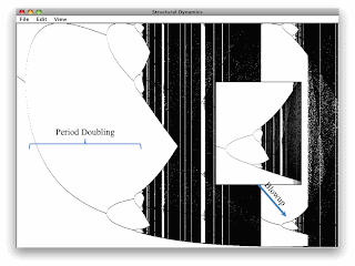
Figures 1 and 2 demonstrate that the limiting behavior of an iterative process for the logistic equation varies with the parameter a. Figure 3 displays this variation from a value of a somewhere under 3.0 to 4.0. In Figure 3, the value of a is plotted along the abscissa. For each value of a, non-transient values of a time series are plotted along the ordinate. To the left of the figure, the time series converges to a single stable limit point. Somewhere to the right, this limit point becomes unstable, and the limiting behavior consists of a cycle of period 2. Moving further to the right - that is, increasing a, limit cycles of period 4, 8, 16, etc. appear. The limit cycle of period 3 shown in Figure 2 corresponds to a parameter value of a somewhere to the center left of the region shown in the blown-up inset.

Figure 3: Structural Dynamics for the Logistic Equation

In some sense, this is recreational mathematics. Computers these days make it fairly easy to draw a more complete representation of Figure 4 in May (1976). The blow-up in Figure 3 demonstrates that the structural dynamics for the logistic function is fractal in nature. We see the same shape repeated on increasingly smaller and smaller scales. Chaos arises for parameter values of a between the period doubling cascade and the period-3 cycle. (Chaotic behavior is shown in Figure 3 by the dark shaded regions.)

3.0 A Exponential-Logistic Equation

I repeated the above analysis for what I am calling an exponential-logistic function:

f₂(x) = (x/c) e^{a(1 - x)}, 0 < a

where:

c = 1, if a - ln a ≤ 1

c = -1/(a e^{a - 1}), if 1 < a - ln a

This exponential-logistic function was suggested to me by a function in May (1976). I introduced the scaling provided by c such that the maximum value of this function never exceeds unity. This function, like the logistic function, is parametrized by a single parameter, which I am also calling a. Figure 4 shows the non-transient behavior for a specific value of the parameter a for the exponential-logistic function. In this case, a stable limit cycle of period 32 arises.

Figure 4: A Cycle with Period 32 for the Exponential-Logistic Equation

Notice the exponential-logistic function is generally not symmetric around any value of x; one tail is heavier than the other. Furthermore, it only has a zero at the origin; nothing corresponds to the zero at x = 1 in the logistic function. So, in some sense, it has a quite different form from the logistic function. Yet, as shown in Figure 5, the structural dynamics for iterative processes for the exponential-logistic function are qualitatively similar to the structural dynamics arising from the logistic function. We see the same shapes in Figures 3 and 5, albeit distorted in some sense.

Figure 5: Structural Dynamics for the Exponential-Logistic Equation

4.0 A Feigenbaum Constant

I now report on some quantitative numerical experiments. Table 1, in the second column, shows the smallest value of the parameter a for which I was able to find a limit cycle of the given period for the logistic equation. Cycles of an infinite number of periods - that is, for all positive integer powers of two (2, 4, 8, 16, ...) - exist in the period-doubling region labeled in Figure 3. As suggested by Table 2, the distance between values of a at which period-doubling occurs gets smaller and smaller. In fact all these limit cycles arise before a = 3.5700..., the point of accumulation of a at which chaos sets in. (I do not fully understand the literature on how to calculate the period of limiting cycles for a. I therefore do not report values of a for larger periods than shown in the table, since I do not fully trust my implementation of certain numeric methods.)

Table 1: Period Doubling in the Logistic Equation

Period	a	Difference	Ratio
2	2.9999078
4	3.4494577	0.449550	4.7510
8	3.5440789	0.094621	4.6556
16	3.5644029	0.020324	4.6669
32	3.5687579	0.004355	4.6665
64	3.5696911	0.000933	4.6666
128	3.5698109	0.000200

Table 1, above shows, in the third column, the difference between values of a at which period-doubling occurs. The fourth column shows the ratio of successive difference. Theoretically, this ratio converges to δ = 4.669201609... My numeric exploration has found this constant to at least two significant figures.

The convergence of this ratio, over limit cycles for periods of powers of two, is not limited to the logistic equation. Table 2 reports the result of a numeric experiment with the exponential-logistic equation. Here too, the constant δ has been found to two significant figures. Interestingly, the ratio would theoretically converge to the same constant if the two tables were infinitely extended. In fact, δ is a universal mathematical constant, like π or e.

Table 2: Period Doubling in the Exponential-Logistic Equation

Period	a	Difference	Ratio
2	2.7180077
4	4.6016740	1.883666	2.9506
8	5.2400786	0.638405	4.2473
16	5.3903856	0.150307	4.5651
32	5.4233107	0.032925	4.6456
64	5.4303982	0.007087

5.0 Conclusion

The above analysis can be generalized to many other functions, albeit I do not fully understand how to characterize the class of such functions. Feigenbaum states that the period doubling route to chaos is not limited to one-dimensional processes. I believe it also arises in continuous time systems, as defined by certain non-linear differential equations. Do you find it surprising that a universal constant with wide applicably to physical processes (like year-by-year changes in the population demographics of certain species), has been discovered in the lifetime of many now alive?

References

• Keith Briggs (1991). A Precise Calculation of the Feigenbaum Constants, Mathematics of Computation, V. 57, No. 195 (July): pp. 435-439.
• Mitchell J. Feigenbaum (1980). Universal Behavior in Nonlinear Systems, Los Alamos Science (Summer): pp. 4-27.
• Tien-Yien Li & James A. Yorke (1975). Period Three Implies Chaos, American Mathematical Monthly, V. 82, No. 10 (Dec.): pp. 985-992.
• Robert M. May (1976). Simple Mathematical Models with Very Complicated Dynamics, Nature, 261: pp. 459-467.

Purge At Amsterdam?

I have noticed that the recent history of economics has been impacted by various purges in various prominent economics departments. I think of, for example, Harvard, Rutgers, and Notre Dame. I had not noticed this one when it was going on:

"For most of my time over ten years at the University of Amsterdam my research and that of my colleagues was strongly supported. (I taught three courses every second fall term, and took leave from Marquette.) Unfortunately over the last two years people in leadership positions there at the faculty of economics decided that the history and methodology of economics (HME) was not important, and in conditions of a financial emergency associated with chronic budget shortfalls closed down the HME group. That included sacking my very accomplished and, in our field, well-respected colleagues Marcel Boumans and Harro Maas, who had been associate professors there for many years, and ending the chair position in HME, which I held, which had been at the faculty for decades. We had six courses in the history and methodology of economics; engaged and enthusiastic students; a research group of up to a dozen people; a master degree in HME; PhD students; and a required methodology course for bachelor students. I do not think there was a better program in the world in our field. We also had great interaction with the London School of Economics, the history of economics people at Duke University, history of economics people in Paris, and the Erasmus Institute for Philosophy and Economics. The HME group was internationally recognized, and attracted students from across the world. Our financial footprint, in fact, was quite small compared to other groups, and by a number of measures of output per person we were more productive than many other research groups at Amsterdam.

Since I fully believe the faculty financial emergency could have been addressed without eliminating the group, I can only put what happened down to prejudice against our field, plus the usual on-going territorial aggrandizing that has been a key factor in the elimination of history of economics from most American universities. It is interesting to me also, that with a few exceptions, members of the economics faculty at Amsterdam made no effort on the HME group’s behalf to resist what happened or even personally expressed regret or concern to those who lost their jobs. I find this reprehensible.

The loss of this program was a blow to our field. There are now few places in the world training PhD students in history and/or methodology of economics. So in the final analysis the situation for economics and philosophy is mixed: considerable achievement with an uncertain future. Great weight, in my view, should be placed on restoring PhD training in the field, something that is being done, for instance, through generous grants from the Institute for New Economic Thinking at Duke University under Bruce Caldwell." -- John B. Davis (2012). Identity Problems: An interview with John B. Davis, Erasmus Journal for Philosophy and Economics, V. 5, Iss. 2 (Autumn): pp. 81-103.

Reminder: Reductionism Is Bad Science

I want to remind myself to try to download the following in a couple of weeks:

Abstract: Causal interactions within complex systems can be analyzed at multiple spatial and temporal scales. For example, the brain can be analyzed at the level of neurons, neuronal groups, and areas, over tens, hundreds, or thousands of milliseconds. It is widely assumed that, once a micro level is fixed, macro levels are fixed too, a relation called supervenience. It is also assumed that, although macro descriptions may be convenient, only the micro level is causally complete, because it includes every detail, thus leaving no room for causation at the macro level. However, this assumption can only be evaluated under a proper measure of causation. Here, we use a measure [effective information (EI)] that depends on both the effectiveness of a system’s mechanisms and the size of its state space: EI is higher the more the mechanisms constrain the system’s possible past and future states. By measuring EI at micro and macro levels in simple systems whose micro mechanisms are fixed, we show that for certain causal architectures EI can peak at a macro level in space and/or time. This happens when coarse-grained macro mechanisms are more effective (more deterministic and/or less degenerate) than the underlying micro mechanisms, to an extent that overcomes the smaller state space. Thus, although the macro level supervenes upon the micro, it can supersede it causally, leading to genuine causal emergence—the gain in EI when moving from a micro to a macro level of analysis. -- Erik P. Hoel, Larissa Albantakis, and Giulio Tononi (2013). Quantifying Causal Emergence Shows that Macro Can Beat Micro, Proceedings of the National Academy of Sciences, V. 110, no. 49.

As far as I can tell, the above article is not specifically about economics. I do not understand download policy for the Proceedings of the National Academy of Sciences. I gather that you must be registered to download articles from the current issues, but can download back issues with no such restriction.

Hat Tip: Philip Ball

Honest Textbooks

1.0 Introduction

Every teacher, I guess, of an introductory or intermediate course has a struggle with how to teach material that requires more advanced concepts, outside the scope of the course, to fully understand. I think it would be nice for the textbooks not to foreclose the possibility of pointing out this requirement. I here provide a couple of examples from some mathematics textbooks that I happen to have.

2.0 Probability

Hogg and Craig (1974) is a book on probability and statistics. I have found many of their examples and theorems of use in a wide variety of areas. They usually do not explain how many of these ideas can be expanded to an entire applied course.

2.1 Borel Sets and Non-Measurable Sets

An axiomatic definition of probability is a fundamental concept for this book. Hogg and Craig recognize that they do not give a completely rigorous and general definition:

Let C denote the set of every possible outcome of a random experiment; that is, C is the sample space. It is our purpose to define a set function P(C) such that if C is a subset of C, then P(C) is the probability that the outcome of the random experiment is an element of C...

Definition 7: If P(C) is defined for a type of subset of the space C, and if,

• P(C) ≥ 0,
• Let C be the union of C₁, C₂, C₃, ... Then P(C) = P(C₁) + P(C₂) + P(C₃) + ..., where the sets C_i, i = 1, 2, 3, ..., are such that no two have a point in common...
• P(C) = 1,

then P(C) is called the probability set function of the outcome of the random experiment. For each subset C of C, the number P(C) is called the probability that the outcome of the random experiment is an element of the set C, or the probability of the event C, or the probability measure of the set C.

Remark. In the definition, the phrase 'a type of subset of the space C' would be explained more fully in a more advanced course. Nevertheless, a few observations can be made about the collection of subsets that are of the type... -- Hogg and Craig (1974): pp. 12-13 (Notation changed from original).

2.2 Moment Generating and Characteristic Functions

Hogg and Craig work with moment generating functions throughout their book. In the chapter in which they introduce them, they state:

Remark: In a more advanced course, we would not work with the moment-generating function because so many distributions do not have moment-generating functions. Instead, we would let i denote the imaginary unit, t an arbitrary real, and we would define φ(t) = E(e^itX). This expectation exists for every distribution and it is called the characteristic function of the distribution...

Every distribution has a unique characteristic function; and to each characteristic function there corresponds a unique distribution of probability... Readers who are familiar with complex-valued functions may write φ(t) = M(i t) and, throughout this book, may prove certain theorems in complete generality.

Those who have studied Laplace and Fourier transforms will note a similarity between these transforms and [the moment generating function] M(t) and φ(t); it is the uniqueness of these transforms that allows us to assert the uniqueness of each of the moment-generating and characteristic functions. -- Hogg and Craig (1978): pp. 54-55.

3.0 Fourier Series

Lin and Segel (1974) provides a case study approach to applied mathematics. They introduce certain techniques and concepts in the course of specific problems. Fourier analysis is introduced in the context of the heat equation. They then look at more generals aspects of Fourier series and transforms. They state:

Suppose that we now pose the following problem, which can be regarded as the converse to Parseval's theorem. Given a set of real numbers a₀, a_m, b_m, m = 1, 2, ..., such that the series

(1/2) a₀² + {[a₁² + b₁²] + [a₂² + b₂²] + ...}

is convergent, is there a function f(x) such that the series

(1/2) a₀ + {[a₁cos(x) + b₁sin(x)]

+ [a₂cos(2x) + b₂sin(2x)] + ...}

is its Fourier series?

An affirmative answer to this question depends on the introduction of the concepts of Lebesque measure and Lebesque integration. With these notions introduced, we have the Riesz-Fisher theorem, which states that (i) the [above] series ... is indeed the Fourier series of a function f, which is square integrable, and that (ii) the partial sums of the series converge in the mean to f.

The problem we posed is a very natural one from a mathematical point of view. It appears that it might have a simple solution, but it is here that new mathematical concepts and theories emerge. On the other hand, for physical applications, such a mathematical question does not arise naturally. -- C. C. Lin & L. A. Segel (1974): p. 147 (Notation changed from original).

4.0 Discussion

Here is a challenge: point out such candid remarks in textbooks in your field. I suspect many can find such comments in many textbooks. I will not be surprised if some can find some in mainstream intermediate textbooks in economics. Teaching undergraduates in economics, however, presents some challenges and tensions. I think of the acknowledged gap between undergraduate and graduate education. Furthermore, I think some tensions and inconsistencies in microeconomics cannot be and are never resolved in more advanced treatments. Off the top of my head, here are two examples.

• The theory of the firm requires the absence of transactions costs for perfect competition to prevail. But under the conditions of perfect competition, firms would not exist. Rather workers would be independent contractors, forming temporary collectives when convenient.
• Under the theory of perfect competition, as taught to undergraduates, firms are not atomistic. Thus, when taking prices as given, the managers are consistently wrong about the response of the market to changes they may each make to the quantity supplied. On the other hand, when firms are atomistic and of measure zero, they do not produce at the strictly positive finite amount required by the theory of a U-shaped average cost curve.

My archives provide many other examples of such tensions, to phrase it nicely.

References

• Robert V. Hogg & Allen T. Craig (1978). Introduction to Mathematical Statistics, 4th edition, MacMillan.
• C. C. Lin & L. A. Segel (1974). Mathematics Applied to Deterministic Problems in the Natural Sciencs, Macmillan

A New Order In Economics From Manchester

Some links:

• The Post-crash Economics Society
• Economics students aim to tear up free-market syllabus, by Phillip Inman, in the Guardian, 24 October 2013.
• Letters: Reconnecting economics and real life, in the Guardian, 25 October 2013.
• Economics students need to be taught more than neoclassical theory, by Zach Ward-Perkins and Joe Earle, in the Guardian, 28 October 2013.
• Mainstream economics is in denial: the world has changed, by Aditya Chakraborthy, in the Guardian, 28 October 2013.
• Economics lecturers accused of clinging to pre-crash fallacies, by Phillip Inman, in the Guardian, 10 November 2013.
• Teaching evidence-based economics, by Michael Joffe, in the Royal Economic Society Newsletter, October 2013.
• University economics teaching to be overhauled, by Phillip Inman, in the Guardian, 11 November 2013.
• Cambridge Society for Economic Pluralism (CSEP)
• Letter to the editor from the Post Keynesian Study Group, 18 November 2013.
• Leter to the editor from the Association for Heterodox Economics, 21 November 2013.
• Keynes's new heirs: Britain leads a global push to rethink the way economics is taught, in the Economist, 23 November 2013.

By the way, Ian Steedman, a leading Sraffian economist, was at the University of Manchester not too long ago. And, I believe, he did supervise a number of doctorate theses from students at Manchester. So the closing of the doors to form the current monoculture happened only over the last decade, I guess.

Update: Originally posted on 6 November 2013. Updated on 12 November 2013 to include more links.

Update: Updated on 2 December 2013 to include more links.