 |
| Figure 1: A Pattern Diagram, Enlarged |
This post looks at and generalizes an example of the recurrence of techniques by Salvatore Barone. It is an example with fixed capital illustrating the recurrence of the period of truncation. In the generalization, I find what I call patterns over the axis for the rate of profits, a patern over the wage axis, a three-technique pattern, and a reswitching pattern.
Barone's example demonstrates that around a switch point, a lower rate of profits can be associated with both an increase and a decrease in the economic life of a machine and an increased life of a machine can be associated with both an increase and a decrease in the capital-intensity of a technique. From other examples, I know the variability in the direction of the period of truncation with the rate of profits, the (non) relationship of the economic life of a machine with output per worker, and the jump (from one years to three) in the economic life of a machine with an infinitesimal variation in the rate of profits are independent of reswitching and capital-reversing.
So much for the Austrian theory of capital.
2.0 TechnologyThe available technology consists of the four processes in Tables 1 and 2. Each process exhibits constant returns to scale (CRS) and takes a year to complete. In the first process, labor and corn are used to make a machine, which, I suppose, I could have called a tractor. In the remaining three processes, labor, corn, and the machine are used to make corn. In each of the first two of these three processes, a machine one year older than it was as an input is jointly produced with corn. Corn is circulating capital and the machine is fixed capital.
| Input | Process | |||
| (I) | (II) | (III) | (IV) | |
| Labor | a0, 1 | a0, 2 | a0, 3 | a0, 4 |
| Corn | a1,1 | a1,2 | a1,3 | a1, 4 |
| New Machines | 0 | 1 | 0 | 0 |
| 1-Year Old Machines | 0 | 0 | 1 | 0 |
| 2-Year Old Machines | 0 | 0 | 0 | 1 |
| Output | Process | |||
| (I) | (II) | (III) | (IV) | |
| Corn | 0 | 1 | 1 | 1 |
| New Machines | 1 | 0 | 0 | 0 |
| 1-Year Old Machines | 0 | 1 | 0 | 0 |
| 2-Year Old Machines | 0 | 0 | 1 | 0 |
I assume that an old machine can be costlessly disposed of before its technical life. Thus, there are three techniques that can arise in a stationary state. In the Alpha technique, the machine is junked after being used one year; only the first two processes are operated. In Beta, the machine is junked after two years. In Gamma, the machine is operated for its full technical life and all four processes are operated.
I conclude this section by specifying parameters for the coeffients of production:
a0, 1 = (2/5) e1 - t/10
a0, 2 = (1/5) e1 - t/10
a0, 3 = (3/5) e1 - t/10
a0, 4 = (2/5) e1 - t/10
a1, 1 = (1/10) e1 - t/10
a1, 2 = (2/5) e1 - t/10
a1, 3 = 0.578 e1 - t/10
a1, 4 = (3/5) e1 - t/10
Barone's example arises when t = 10. The exponential decay in these coefficients is a description of technical progress as exogeneous.
3.0 Prices of ProductionI now want to consider prices of production, given the technology at a point of time, specifically for Baldone's example. I take corn as numeraire. For a given technique, each operated process provides an equation. I take labor as advanced and assume wages are paid out of the end of the year. Given the rate of profits, one can then solve for the wage and the prices of a new machine, a one-year old machine, and a two-year old machine.
Figure 2 plots the wage curves for the three techniques. (By the way, Baldone has a transcription error in at least one of his equations. I was able to replicate his tables with this error corrected.) The cost-minimizing techniques are noted, even though which is on the outer frontier is not always easily visible.
 |
| Figure 2: The Wage Frontier in Baldones Example |
Figure 3 shows the price of a new machine. At a switch point point, prices are identical for the techniques whose wage curves intersect at that switch point. For example, a rate of profits of approximately 4 percent, the price of a new machine for the Alpha and the Gamma technique is the same.
 |
| Figure 3: The Price of a New Machine |
Figure 4 is finally an example which is visually obvious. The price of an old machine is zero for a technique in which that machine is not produced. Figure 4 shows the prices of only those old machines that are produced in the corresponding technique. In an analysis of the choice of technique with fixed capital, if the price of an old machine is negative at a given rate of profits, the cost minimizing technique must have the economic life of machine must be truncated.
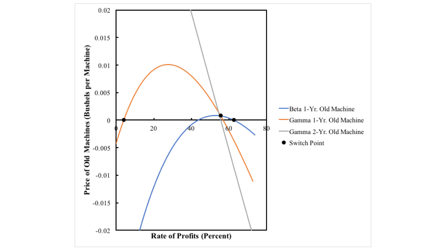 |
| Figure 4: The Price of Old Machines |
Consider, for example, rates of profits less than approximately 4 percent or greater than approximately 63 percent. The price of a one-year old machine under the Beta technique is negative. The prices of one-year old and two-year old machines under the Gamma technique are both negative. Thus, neither can be cost-minimizing. The Alpha technique must be cost-minimizing in these ranges of the rates of profits.
At a rate of profits of approximately 56 percent, the price of a one-year old is positive and the same for the Beta and Gamma techniques, and the price of a two-year old machine is zero under the Gamma technique. This is a switch point for the Beta and the Gamma technique. The price of a two-year old machine is negative under the Gamma technique for any rate of profits greater than this. The Gamma technique cannot be cost-minimizing between 56 and 63 percent. Since the price of a new machine and a one-year old machine is positive, in this range, under the Beta technique, it is not cost-minizing to truncate the machine to an economic life of one year. By the same logic, it is not cost-minimizing to truncate the machine at all for rates of profits between 4 percent and 56 percent.
The analysis of the choice of techniques based on prices yields the same conclusions as an analysis based on the construction as the outer wage frontier. Table 3 summarizes characteristics of the Baldone example. The switch point at approximately 56% is the only one of the three that is not 'perverse'. Around this switch point, a lower rate of profits is associated with an increase in the economic life of the machine, a greater capital-intensity, and more output per worker.
| 0 ≤ r ≤ 4.066% | Alpha cost minimizing. |
| r ≈ 4.066% | Lower rate of profits associated with a decrease in the economic life of the machine, from three years to one year. Consumption per worker increased. |
| 4.066% ≤ r ≤ 55.656% | Gamma cost-minimizing. |
| r ≈ 55.656% | Lower rate of profits associated with an increase in the economic life of the machine, from two to three years. Consumption per worker increased. |
| 55.656% ≤ r ≤ 62.732% | Beta cost-minimizing. |
| r ≈ 62.732% | Lower rate of profits associated with an increase in the economic life of the machine, from one to two years. Consumption per worker decreased. |
| 62.732% ≤ r ≤ 74.166% | Alpha cost minimizing. |
4.0 An Extension for Structural Dynamics
I now introduce structural dynamics. I let all coefficients of production for inputs of labor and corn decrease exponentially, at a rate of 10%. Figure 5 illustrates how the variation of the cost-minimizing technique with the rate of profits changes with technical progress. Here, the economy is not viable at the initial time. There must be some sort of low-productivity, backstop technology that was previously used. Figure 5 partitions time into six regions, and Figure 1, at the top of this post enlarges transient regions. Baldone's example is in Region 3.
 |
| Figure 5: A Pattern Diagram |
5.0 Conclusion
I suppose I should figure out a complete characterization of all six regions, not just Region 3. I now have more examples with fixed capital for my approach to structural economic dynamics than can be comfortably be described in a paper of reasonable length.
I am finding that the analysis of so-called 'paradoxes' in models of the prices of production with fixed capital is an important extension of the Cambridge Capital Controversy. A thorough understanding of the 13-page Chapter X in Sraffa's book only became available in English after mainstream economists had commenced on ignoring certain results.
References- Salvatore Baldone. 1974. Il capitale fisso nello schema teorico di Piero Sraffa. Studi Economici XXIV(1): 45-106. Translated in Pasinetti (1980).


2 comments:
Looking at this example one would wonder about the depreciation of machines. Specifically if depreciation is radioactive or just decreasing if it is linear or monotonic as well as non monotonic and age-dependent or independent from the capital-labour ration. The use of exponential decreasing of inputs also would give rise to snapshots with constant efficiency as well as equal proportions. In these particular Region 4 looks like a candidate for equal proportions but not just that exponential function can be tweaked to give continuous equal proportions of differential rates of radioactive depreciations.
https://www.deepdyve.com/lp/wiley/depreciation-of-machines-of-changing-efficiency-a-note-W17V4n4w29?articleList=%2Fsearch%3Fquery%3Dian%2Bsteedman%26sort%3Doldest
https://books.google.es/books?hl=en&lr=&id=CQayCwAAQBAJ&oi=fnd&pg=PA65&ots=nou8O4_V4J&sig=j5p1XCid3crVz9U6zQtxcyOwK2Q&redir_esc=y#v=onepage&q&f=false
https://www.deepdyve.com/lp/springer-journals/durable-capital-inputs-conditions-for-price-ratios-to-be-invariant-to-MjI9KqqX0o?articleList=%2Fsearch%3Fquery%3Dsamuelson%2Bcapital%2Bdurable
https://www.deepdyve.com/lp/springer-journals/durable-capital-inputs-conditions-for-prices-ratios-to-be-invariant-to-xnSvaGrQkJ?articleList=%2Fsearch%3Fquery%3Dsamuelson%2Bcapital%2Bdurable
https://www.deepdyve.com/lp/wiley/differential-depreciation-and-the-2-2-model-of-distribution-pricing-OeA8OfCWIF?articleList=%2Fsearch%3Fquery%3Dian%2Bsteedman%26page%3D3%26sort%3Doldest
I would try to generalise this example to obtain equal proportions and equal proportions with constant efficiency of machines, even if that swipes truncation away.
Post a Comment