Greg Mankiw Should Try To Make A Honest Living

A Discussion On The Best (or Worst) Of Mankiw

Peter Bofinger has expanded a series of tweets to point out some stuff that is just wrong in Mankiw's introductory textbook. The video above is a virtual panel discussion in which Mankiw graciously pretends to respond to Bofinger. Rüdiger Bachmann and Anna Reisch also participate. I do not know the host, Thomas Fricke. Questions from the audience are fielded towards the end. I concentrate on Sascha Buetzer (1:07:45) below. Other questions are from Janina Urban (1:18:41) and Thomas Kopp (1:21:29). I am probably missing something.

I wonder whether Anna Reisch knows about Adolph Lowe's political economics. I know of this through his 1965 book On Economic Knowledge. I gather Lowe thought it was the task of economists to say whether a given end state is internally consistent and to explain how it could be reached.

I want to point out some hypocrisy from Mankiw. He does not even bother arguing that Bofinger has pointed out confusion and nonsense in his textbook. He says that he sees his job as presenting the consensus of mainstream economics, not his own theories. He tries to minimize the imposition of his own idiosyncrasies. Now Buetzer is, if I hear correctly, the senior advisor to the German director to the International Monetary Fund (IMF). Buetzer offers the difficult proposition that "textbooks should strive to be factually correct." And one of his points is that, "all modern empirical evidence ... point to ... there is no equity-efficiency tradeoff from moderate levels of redistribution, but rather the opposite." This is the "mainstream in mainstream institutions". Does Mankiw say he will then update his textbook in the next edition to reflect the mainstream view? Of course not. He starts presenting his own idiosyncratic reasons for rejecting empirical evidence.

Economists should strive not to teach falsehoods and nonsense and not to promote the teaching of falsehoods and nonsense. Maybe Mankiw is correct that if he discarded from his textbooks stuff that is, at best, just wrong, his textbooks would not sell as well. That is no justification for retaining balderdash. Although Mankiw may disagree, he is not entitled to an income from textbooks.

On The Empirical Verification Of The Cambridge Capital Controversy

1.0 Introduction

My consistent position is that Sraffa and his followers, besides recovering an alternate approach to value and distribution found in classical economics and Marx, demonstrated the logical invalidity of marginalist economics. Empirical results are irrelevant to questions of logical validity.

Wage curves, as constructed from input-output matrices, are rational functions with the numerator and denominator both being some high order polynomial functions. I would have liked to see some more wobbles in those constructed empirically and more examples of reswitching and capital-reversing. Nevertheless, the finding that frontiers are close to linear functions, with only a few switch points, is not consistent with an emphasis on widespread marginal adjustments. It is more consistent with Marx's theory of value and Joan Robinson's understanding of technical change, in which the question of the choice of technique at a given moment in time is, at most, a secondary concern. Schefold's recent work (Schefold 2013, Schefold 2016, Götz and Schefold 2020) with random matrices is of interest here for trying to explain the empirical posts.

I have written about empirical results before. In this post I concentrate on Zambelli (2018) as the most recent, most extensive empirical examination of input-output matrices. See also the comments on Zambelli's work in Götz and Schefold (2020).

2.0 Progress in Empirical Research Work

Increased computer power and more complete consistent national income and product accounts (NIPAs) has supported empirical research. If I recall correctly, Ochoa (1987) looks at wage curves as based on input-output matrices from different times. He looks for pairs that intersect more than onec.

In looking at such a pair, however, many more wage curves are available. One can construct input-output matrices, with one process for each industry, where the processes are not all from one matrix but combine processes among industries from the different matrices. Han and Schefold (2006) take this approach.

But this is not all. One need not limit oneself with processes from pairs of wage curves. One should look at the full range of techniques, where the process for each industry might be from any input-output matrix in your database. Zambelli (2018), in following this approach, uses an algorithm that he and his colleagues cleverly constructed to select the wage curves on the frontier, thereby keeping the combinatorial explosion in this approach somewhat under control.

Ideally, one would like internationally consistent classifications of industries in make and use tables and Leontief input-output matrices that include joint production. If the latter is not available, which it usually not, one needs consistent approximations for single-production. Since make and use tables, and the resulting Leontief input-output tables are typically price data, one needs price indices for industries or commodities. At what level of aggregation do some industries only appear in some tables? Many more questions arise here that are probably beyond me.

3.0 'Perverse' Phenomena

What supposedly 'perverse' phenomena should one look for in techniques formed out of empirical input-output matrices? I suggest instances of the reswitching of techniques, capital reversing, the reverse substition of labor, and the recurrence of processes in individual industries would be of interest. Reswitching on the frontier is sufficient, but not necessary for the occurrence of positive real Wicksell effects. I, like many others, define capital reversing (also known as reverse capital deepening) as equivalent to positive real Wicksell effects. Zambelli (2018), on the other hand, defines capital reversing to arise with positive real or price Wicksell effects.

I tend, in pointing out the invalidity of marginalist economics, to de-emphasize any concern with the direction of price Wicksell effects. As I understand it, the direction of price Wicksell effects is dependent on the selection of the numeraire. Also, I am aware of Burmeister's championing of Champernowne's chain index for capital. On the other hand, Baldone (1984) suggest this defense of mainstream economics fails. Fratini (2010) has an example with a continuous variation of techniques along the wage frontier and in which negative price Wicksell effects swamp positive real Wicksell effects, which I guess is a propos here.

4.0 Wage Frontiers and Aggregate Production Functions

I have been talking about wage frontiers and wage curves above. One can construct the aggregate production 'function', given the analysis of the choice of technique. In this analysis, one takes net output as of a given physical composition. It is convenient to take net output as the numeraire. The composition of capital goods varies at switch points, and their prices vary between switch points. At one point, though, Zambelli considers variations in the composition of capital goods between switch points, as I understand it. I relegate an explanation of what he is doing here to an appendix.

5.0 Conclusion

Zambelli (2018) is impressive empirical work. The failure of so-called neoclassical theory in 60 percent of the cases examined, as I understand it results, from a concentration on price Wicksell effects, which would not disconcert, for example, Burmeister. I also have difficulties with how Zambelli relates the aggregate production function to a problem of minimizing the value of aggregate capital.

Appendix: The Construction of a Microeconomic Production Function

I illustrate the construction of a production funcition as the solution of a maximization problem. A more general presentation would start with netput vectors and assume convexity. I briefly glanced at the appendix to chapter VI in Pasinetti (1977) in writing this.

For concreteness, suppose the managers of a firm have given quantities, x₁, x₂, and x₃, of three resources and know of four fixed-coefficient processes for producing a single commodity. The coefficicients of production for these four processes are:

(a_.j)^T = (a_{1, j}, a_{2, j}, a_{3, j}), j = 1, 2, 3, 4.

Let q_i, i = 1, 2, 3, 4, be the decision variables denoting how much output is produced with each process. Consider the linear following linear program (LP). Maximize output y:

y = q₁ + q₂ + q₃ + q₄

such that:

a_{1, 1} q₁ + a_{1, 2} q₂ + a_{1, 3} q₃ + a_{1, 4} q₄ ≤ x₁

a_{2, 1} q₁ + a_{2, 2} q₂ + a_{2, 3} q₃ + a_{2, 4} q₄ ≤ x₂

a_{3, 1} q₁ + a_{3, 2} q₂ + a_{3, 3} q₃ + a_{3, 4} q₄ ≤ x₃

q_i ≥ 0, i = 1, 2, 3, 4 = 1, 2, 3, 4.

The constraints express the condition that no more of a resource (also known as a factor of production) can be used than is given. Every process must be operated at a non-negative level. Let f express the solution of this LP as a function of factors of production:

y = f(x₁, x₂, x₃)

This is a discrete version of the production function for a given commodity. It has properties commonly assumed in marginalist economics. It exhibits constant returns to scale (CRS) and non-increasing marginal products. If one wanted to construct a production function differentiable everywhere, one could assume an uncountably infinite set of production processes.

I might as well write down the dual problem. It is to choose factor prices w₁, w₂, w₃ to minimize:

w₁ x₁ + p₂ x₂ + p₃ x₃

such that:

a_{1, 1} w₁ + a_{2, 1} w₂ + a_{3, 1} w₃ ≥ 1

a_{1, 2} w₁ + a_{2, 2} w₂ + a_{3, 2} w₃ ≥ 1

a_{1, 3} w₁ + a_{2, 3} w₂ + a_{3, 3} w₃ ≥ 1

a_{1, 4} w₁ + a_{2, 4} w₂ + a_{3, 4} w₃ ≥ 1

w₁ ≥ 0, w₂ ≥ 0, w₃ ≥ 0

For a solution of these two LPs, the values of their objective functions are equal. Factor prices are such that output is completely distributed among the owners of the resources whose services are used in producing the given commodity. If a constraint in the dual is met with inequality, the corresponding decision variable in the primal LP is set to zero. That process is not operated. If a constraint in the primal LP is met with an inequality, that resource is in excess supply and its price is zero. Even though you see no derivatives above, this is an exposition of an aspect of the theory of marginal productivity.

All the parameters and variables in the primal LP are in physical units (for example, bushels, tons, person-years). It does not make much sense to me in an aggregate production function, with output and arguments in price terms, to maximize the value of output for a given value of capital or to minimize the value of capital for a given value of output. Nevertheless, that is what Zambelli does in Section 5.3 of his paper. I suppose he wanted to present a comprehensive empirical exploration of aggregate neoclassical theory, taking its illogic as given.

References

• Baldone, Salvatore. 1984. From surrogate to pseudo production functions. Cambridge Journal of Economics 8: 271-288.
• Burmeister, E. 1980. Capital Theory and Dynamics. Cambridge: Cambridge University Press
• Fratini, Saverio M. 2010. Reswitching and decreasing demand for capital. Metroeconomica 61 (4): 676-682.
• Han, Zonghie and Bertram Schefold. 2006. An empirical investigation of paradoxes: reswitching and reverse capital deepening in capital theory. Cambridge Journal of Economics 30: 737-765.
• Kersting, Götz and Bertram Schefold. 2020. Best techniques leave little room for substitution: a new critique of the production function. Centro Sraffa Working Paper n. 47.
• Ochoa, E. M. 1987. Is reswitching empirically relevant? US wage-profit-rate frontiers, 1947-1972. Economic Forum 16: 45-67.
• Pasinetti, Luigi L. 1977. Lectures on the Theory of Production New York: Columbia University Press.
• Schefold Bertram. 2013. Approximate surrogate production functions. Cambridge Journal of Economics 37 (5): 1161-1184.
• Schefold Bertram. 2016. Profits equal surplus value on average and the significance of this result for the Marxian theory of accumulation.. Cambridge Journal of Economics 40 (1): 165-199.
• Zambelli, Stefano. 2018. The aggregate production function is NOT neoclassical. Cambridge Journal of Economics 42: 383-426.

Books To Make You More Muddled

I have not read all of these, and you might think I am being unfair with this post title. If you want critiques of post modernism, try the Amin and Eagleton referenced at the end of this post. Sokal, after the cited book, participated in interesting colloquia with those who were scholars of what he was attacking and mocking. If you want to see how little I know about this area, you can look at my posts on Gramsci, Foucault, Wittgenstein, or Zizek.

• Gellner, Ernest. 1959. Words and Things: A Critical Account of Linguistic Philosophy and a Study in Ideology. London: Gollantz.
• Gross, Paul R. and Norman Levitt. 1998. Higher Superstition: The Academic Left and its Quarrels with Science. Baltimore: John Hopkins Press.
• Hicks, Stephen R. C. 2004. Explaining Postmodernism: Skepticism and Socialism from Rousseau to Foucault. New Berlin: Scholarly Publishing.
• Pluckrose, Helen and James A. Lindsay. 2020. Cynical Theories: How Activist Scholarship Made Everything about Race, Gender, and Identity - and Why This Harms Everybody. Pitchstone Publishing.
• Sokal, Alan and Jean Bricmont. 1998. Fashionable Nonsense: Postmodern Intellectuals Abuse of Science. New York: Picador USA.

John Roemer's Reproducible Solution

Can I adapt Roemer's work, suitably taking into account later work by D'Agata and Zambelli, to found this approach to markup pricing? As a start, I here quote Roemer on a reproducible solution (RS), before he takes into account unequal rates of profits and a choice of technique. Given the role of endowments, is this a neoclassical approach, like Hahn's 1984 CJE paper? Even so, is it a valid justification for Sraffa's price equations? Notice there are no subscripts for time below.

"There are N capitalists; the νth one is endowed with a vector of produced commodity endowments ω^ν ... Capitalist ν starts with capital ω^ν, which he seeks to turn in more wealth at the highest rate of return. Thus the program of capitalist ν is

Facing prices p, to

choose x^ν ≥ 0 to

max (p - (p A + L)) x^ν

s.t. (p A + L) x^ν ≤ p ω^ν

(The constraint says that the inputs costs can be covered by current capital.) Let us call A^ν(p) the set of solution vectors to this program." -- Roemer (1981: 18-19, I made changes for typesetting mathematics).

Roemer defines a RS:

"Definition 1.1: A price vector p is a reproducible solution for the economy {A, L; b; ω¹, ..., ω^N} if:

• For all ν, there exists x^ν in A^ν(p), such that (profit maximization)
• x = Σ x^ν and x ≥ A x + (L x) b (reproducibility)
• p b = 1 (subsistence wage)
• A x + (L x) ≤ ω = Σ ω^ν (feasibility)

We shall also refer to the entire set {p, x¹, ..., x^N} as a reproducible solution." -- Roemer (1981: 19-20, with for math).

A RS can only exist if the elements of the endowment vector are in certain proportions:

"Theorem 1.2: Let the model {A, L, b} be given with A productive and indecomposable, and the rate of exploitation e > 0. Let {p, x¹, ..., x^N} be a nontrivial RS. (i.e., Σ x^ν = x ≠ 0). Then the vector of prices p is the E[qual] P[rofit] R[ate] vector p^*. Furthermore, a RS exists if and only if omega is an element of C^*, where C^* is a particular convex cone in [the space of n-dimensional real vectors] containing the balanced growth path of {A, L, b}. (C^* is specified precisely below.)" -- Roemer (1981: 20, with changes for math).

Even though endoments are taken as given in defining the firm's LP, endowments are endogenous in the sense that they must lie close to those on a balanced growth path. I like to have labor advanced and wages paid out of the surplus, instead of vice versa as above. The above does not allow for a choice of technique. Roemer has at least some of this in later chapters.

References

• John E. Roemer. 1981. Analytical Foundations of Marxian Economic Theory. Cambridge University Press.

23 February 1981: King Juan Carlos Becomes A Spanish National Hero

I only know about this at the level of a Wikipedia article. Or maybe a short newspaper article. Some of you doubtlessly know more.

Some Spanish military officers, pining for the certainty of a fascist authortarian state, assaulted the Congress of Deputies in 1981. They held the deputies hostage. Some showed real physical courage. The prime minister and deputy prime minister refused to sit down when ordered so, despite having guns pointed at them.

I'd like to conclude that, despite this failed coup attempt, Spain is a thriving democracy today. But I think political parties today are addressing problems more connected with austerity after 2008 than with nostalgia for Franco. I conclude with a couple references about violence in politics.

• Hannah Arendt. 1969. On violence. In Crises of the Republic New York: Harcourt Brace Jovanovich.
• Georges Sorel. 1950. Reflections on Violence (Trans. by T. E. Hulme) London: Collier-Macmillan.

The Tractor-Corn Model: A Start

1.0 Introduction

In my ROBE article, I consider fluke switch points arising from perturbations of coefficients of production in the Samuelson-Gargenani model, but in the case with only circulating capital. An obvious generalization is to consider fixed capital. This generalization is simplified by restricting oneself to the case in which machines operate with constant efficiency. Steedman (2020) analyzes this case, and this post is a start on working through elements of the corn-tractor model he leaves as homework. I do not know how far I will go in rewriting my paper for this case.

2.0 Technology for a Technique

In the model, corn is produced by labor working working with a specified type of tractor. And that type of tractor is itself produced by labor working with that type of tractor.

Each type of tractor defines a technique, where a technique is specified by six parameters:

• a: The number of tractors (of a given age) whose services are used for a year in producing a new tractor.
• b: The person-years of labor needed to work with tractors (of a given age) to produce a new tractor.
• n: The number of years a tractor lasts when used in producing new tractors.
• α: The number of tractors (of a given age) whose services are used for a year in producing a bushel of corn.
• β: The person-years of labor needed to work with tractors (of a given age) to produce corn.
• ν: The number of years a tractor lasts when used in producing corn.

The notation is Steedman's, borrowed from J. R. Hicks. I see that if I keep this notation, I will have to drop my usual practice, in honor of Joan Robinson, of using lowercase Greek letters to refer to a technique.

Consider, for a technique, the (n + ν)-element row vector of labor coefficients a₀, the (n + ν) x (n + ν) matrix A of input coefficients, and the (n + ν) x (n + ν) matrix B of output coefficients. This vector and these matrices have a block structure:

a0 =

b

b (uT)1,n - 2

b

β

β (uT)1,ν - 2

β

A =	0	01,n - 2	0	0	01,ν - 2	0
	a	01,n - 2	0	α	01,ν - 2	0
	0n - 2, 1	a In - 2,n - 2	0n - 2, 1	0n - 2,1	0n - 2,ν - 2	0n - 2,1
	0	01,n - 2	a	0	01,ν - 2	0
	0ν - 2,1	0ν - 2,n - 2	0ν - 2,1	0ν - 2,1	α Iν - 2,ν - 2	0ν - 2,1
	0	01,n - 2	0	0	01,ν - 2	α

B =	0	01,n - 2	0	1	(uT)1,ν - 2	1
	1	(uT)1,n - 2	1	0	01,ν - 2	0
	a	01,n - 2	0	0	01,ν - 2	0
	0n - 2,1	a In - 2,n - 2	0n - 2, 1	0n - 2, 1	0n - 2,ν - 2	0n - 2, 1
	0	01,n - 2	0	α	01,ν - 2	0
	0ν - 2,1	0ν - 2,n - 2	0ν - 2,1	0ν - 2,1	α Iν - 2,ν - 2	0ν - 2,1

Obviously, HTML defeated me here. I is the identity matrix, and u is a column unit vector.

Each element of a₀ and each column of A and B correspond to a process of production. The first n columns constitute the tractor sector, and the remaining ν columns are the corn sector. I assume constant returns to scale and that each process requires a year to complete. a_{0, j} is the person-years of labor that enters the jth process per unit-level of operations. The jth column of A is the inputs consumed by the process, and the jth column of B is the outputs. The first row index is for corn. The first row of A is zero, since corn is not used as an input in any process. The second row index is for new tractors. The remaining row indices are for old tractors. Once a tractor is used in tbe production of tractors, it can no longer be used in producing corn. Likewise, a tractor used in the corn sector cannot be transferred to the tractor sector.

3.0 An Annuity

Consider an annuity c_n(r) bought for a dollar at the start of a year. This annuity pays out the sum c_n(r) at the end of the first year, at the end of the second year, and so on through the end of the nth year. This arrangement implicitly specifies an interest rate r which equates the cost and the present value of the payments:

1 = c_n(r)/(1 + r) + c_n(r)/[(1 + r)²] + ... + c_n(r)/[(1 + r)ⁿ]

A bit of algebra reveals that the payments for the annuity are given by the following formula:

c_n(r) = r (1 + r)ⁿ/[(1 + r)ⁿ - 1]

The limit as the interest rate approaches zero can be found by L'Hôpital's rule. It is:

c_n(0) = 1/n

I need these formulas below.

4.0 The Quantity System

Now I want to consider a steady state in which the economy grows at a uniform rate of 100 g percent. Let the column vector q specify the level of operation of each process. I postulate that q has the following form:

q^T = [q₁, q₁/(1 + g), ..., q₁/(1 + g)^{n - 1}, q₂, q₂/(1 + g), ..., q₂/(1 + g)^{ν - 1}]

where q₁ and q₂ are variables to be determined. Let e₁ be the first column of the identity matrix. Consumption in a steady-state is c(g) e₁, where:

c(g) e₁ = [B - (1 + g) A] q

Expanding the first element of the column vectors on both sides, one gets:

c(g) = (1 + g) q₂/c_ν(g)

The second element yields:

0 = {[(1 + g)/c_n(g)] - (1 + g) a} q₁ - (1 + g) α q₂

Or:

0 = [1 - a c_n(g)] q₁ - α c_n(g) q₂

Given g, the above is a linear equation in q₁ and q₂. New tractors do not enter into consumption. Quantity flows are specified such that one person-year of labor is employed:

a₀ q = 1

Or:

(1 + g) b q₁/c_n(g) + (1 + g) β q₂/c_ν(g) = 1

Or:

b c_ν(g) q₁ + β c_n(g) q₂ = c_n(g) c_ν(g)/(1 + g)

A linear system of two equations in two unknowns, given the rate of growth, has now been derived.

The system is easily solved:

q₁ = α c_n(g) c_ν(g) /{[β + αbc_ν(g) - aβc_n(g)](1 + g)}

q₂ = [1 - ac_n(g)] c_ν(g)/{[β + αbc_ν(g) - aβc_n(g)](1 + g)}

Consumption per worker (in units of bushels corn per person-year) is:

c(g) = [1 - ac_n(g)]/[β + αbc_ν(g) - aβc_n(g)]

In a comparison of steady states, consumption per worker is higher if the rate of growth is lower. The dependence of the denominator on the rate of growth vanishes under the special case in which:

a c_n(g)/b = α c_ν(g)/β

Somehow, the above says that the organic composition of capital does not vary between the tractor and the corn sectors. The tradeoff, however, between consumption per worker and the rate of growth is still not linear. The maximum rate of growth, G, is the smallest non-negative real solution to:

0 = 1 - a c_n(G)

Consumption per worker in a stationary state is:

c(0) = [n - a]ν/[nνβ + αbn - aβν]

One might use the above to discuss the capital-intensity of a technique. If the technique with one type of tractor is more capital-intensive than the technique with another type, one would expect c(0) to be higher with the first type.

5.0 The Price System

I now consider prices. Let p be a row vector of prices, w the wage, and r the rate of profits. In matrix form, the price equations are:

p A (1 + r) + w a₀ = p B

A bushel corn is the numeraire:

p e₁ = 1

The above consists of a system of (n + ν + 1) equations for (n + ν + 2) variables. The system has one degree of freedom. Labor is advanced, and wages are paid out of the surplus at the end of the year. A tractor of each age and history has a seperate price.

I now rewrite the price equations for the first time. The price of a bushel cotn is unity, and p represents thd price of a new machine. p_m,j is the price of a j-year old tractor in the tractor sector. p_c,j is the price of a j-year old tractor in the corn sector. The n equations for the tractor sector are:

p a (1 + r) + w b = p + p_m,1 a

p_m,1 a (1 + r) + w b = p + p_m,2 a

...

p_{m,n - 1} a (1 + r) + w b = p

The ν equations for the corn sector are:

p α (1 + r) + w β = 1 + p_c,1 α

p_c,1 α (1 + r) + w β = 1 + p_c,2 a

...

p_{c,ν - 1} α (1 + r) + w β = 1

Consider the equations for the machine sector. Multiply the first equation by (1 + r)^{n - 1}, the second equation by (1 + r)^{n - 2}, and so on, until the last equation is multiplied by (1 + r)⁰.Sum these equations:

p a (1 + r)ⁿ + w b [1 + (1 + r) + ... + (1 + r)^{n - 1}] = p [1 + (1 + r) + ... + (1 + r)^{n - 1}]

The prices for old tractors appear on both sides of successive equations with the same coefficient and drop out. A similiar procedure for the corn sector yields:

p α (1 + r)^ν + w β [1 + (1 + r) + ... + (1 + r)^{ν - 1}] = [1 + (1 + r) + ... + (1 + r)^{ν - 1}]

So far, this procedure works if tractors do not have constant efficiency. The next step requires that, though. The price equations become:

p a c_n(r) + w b = p

p α c_ν(r) + w β = 1

Fpr both the quantity and the price system, a set of (n + ν) equations is reduced to two equations in which (quantities or prices) of old tractors do not enter. The charge for a tractor is that of an annuity that pays out for each year of the tractor's life.

The price system is easily solved. The price of a new tractor is:

p = b/[β + αbc_ν(r) - aβc_n(r)]

Under the special case of equal organic compositions of capital, the ratio of a price of a new tractor to a bushel corn is the ratio of direct labor inputs. Presumably, prices are also proportional to labor values in this special case. The wage curve is:

w = [1 - ac_n(r)]/[β + αbc_ν(r) - aβc_n(r)]

I have already discussed the wage curve under the guise of the tradeoff between consumption per worker and the rate of growth. The maximum rate of profits R is identical to the maximum rate of growth G.

6.0 Conclusion

Steedman (2020) avoids writing about almost all of the above or leaves it as an exercise for the reader. Basically, I have derived Steedman's first five numbered equations. Some of this is in Chapter 10 of Sraffa (1960).

References

• Gargenani, Pierangelo. 1970. Heterogeneous capital, the production function and the theory of distribution. Review of Economic Studies 37 (3): 407-436..
• Samuelson, Paul A. 1962. Parable and realism in capital theory: the surrogate production function. Review of Economic Studies 29 (3): 193-206.
• Steedman, Ian. 2020. Fixed capital in the corn-tractor model. Metroeconomica 71: 49-56.
• Vienneau, Robert L. 2018. Normal forms for switch point patterns. Review of Behavioral Economics 5 (2): 169-195.

The Truncation Of The Economic Lives Of Machines

'Paradoxes' and 'Perversities'

Phenomenon	Example	Region
Reswitching	'One good'	5
	Schefold reswitching	3
	Schefold roundabout	3
	Baldone	8
Recurrence of technique (without reswitching)	Baldone	9
Recurrence of truncation (without reswitching or recurrence of technique)	Two sectors with fixed capital	2
Non-monotonic variation of economic life of machine (without reswitching or recurrence of technique or of truncation)	Baldone	10
'Non-continuous' variation in economic life of machine associated with infinitesimal variation in rate of profits	'One good'	1, 5
	Baldone	7, 8, 9, 10, 11
Increased economic life of machine associated with lower capital intensity	'One good'	1, 3, 4
	Schefold reswitching	2
	Two sectors with fixed capital	1, 2, 3, 4
	Baldone	9, 10, 11
A lower rate of profits associated with a decreased economic life of a machine	'One good'	1, 3, 4, 5
	Schefold reswitching	2, 3
	Two sectors with fixed capital	1, 2, 3, 4
	Baldone	8, 9, 10, 11
Decreased roundaboutness associated with a lower rate of profits	Schefold roundabout	2, 3, 4

I have been exploring simple models of fixed capital, of the production of commodities with machines that last more than one production period. And in these models, the efficiency of machines varies with age. An older machine might require greater care or produce more of a finished commodity after it has been broken in. The choice of technique becomes a question of the choice of the economic life of a machine. In the jargon, managers of firms decide on whether to truncate the use of machine and for how long.

One might think intuitively, but wrongly, that by first producing a machine and then using it in the production of a finished good that one was adopting a more capital-intensive technique than by directing producing the finished good. Likewise, one might wrongly believe that extending the economic life of a machine increases the capital-intensity of a technique. And that a lower rate of interest (or a higher wage) provides incentives to the managers of firms to adopt more capital-intensive techniques.

One can see that these beliefs are incorrect by looking at specific numerical examples. The table at the head of this post provides examples of curious phenomena seen for the fixed capital. Links are provided to specific examples. (The numbering of regions for the 'one good' example are not consistent over the years that I have been working on models of fixed capital.) I think that some of these effects have not been noted in the literature before, albeit I always suspect that Kurz and Salvadori's 1995 textbook might have a homework problem that I now understand the point of.

The truncation of machines is another aspect of the Cambridge Capital Controversy (CCC). But it was not made much of during the 1960s.

My research project of looking at parameter perturbations to identify fluke switch points and partitions of parameter spaces is hardly exhausted. Some research areas to investigate include:

• Create and perturb examples of reswitching and capital reversing, for example, in models of fixed capital in which machines operate with constant efficiency.
• Perturb coeficients of production and requirements for use in models with land, paying particular attention to the order of efficiency, the order of rent, extensive rent, and intensive rent.
• Perturb coefficients of production and requirements for use in general models of joint production.
• Revisit the above considering perturbations of relative markups among industries, instead of coefficients of production.
• Develop computer programs to aid in these analyses.

And besides extending my results, I still need to make an effort to submit much of what I have for publication.

I have decided that applying these results in sensitivity studies of empirical results with National Income and Product Accounts (NIPAs) is probably beyond me. One might consider how perturbations and fluke switch points relate to specific types and biases of technical change. And one might state mathematical theorems and provide proofs.

More On Baldone Example

Figure 1: A Two-Dimensional Pattern Diagram, Enlarged

1.0 Introduction

This post further generalizes an example from Salvatore Baldone.. Like an example from Bertram Schefold, I find that Baldone's example is in a wedge near the edge of the appropriate region in one of my partitions of a parameter space. I have some very complicated spreadsheets that allow me to quickly visualize the effects of varying parameters. Baldone and Schefold were working long before Visicalc, Microsoft Excel, or LibreOffice. Finding these numeric examples must have been tedious.

I think Baldone created this example to illustrate recurrence of truncation. Recurrence of truncation does not necessarily require the recurrence of techniques, but in this example recurrence of truncation occurs with recurrence of techniques. I found it interesting that I could also find here a non-monotonic variation of the economic life of a machine, without recurrence of techniques or capital-reversing.

2.0 Technology

Tables 1 and 2 specify the processes available in this economy. In the first process, labor works with corn to produce a new machine. In the remaining three processes, labor works with corn and a machine to produce corn. A machine one year older than the machine used as an input is jointly produced with corn. Prices of production are defined for coefficients of production at a given moment in time. Technical progress leads to coefficients of production for inputs declining over time. The notation allows for technical progress to be at different rates in the machine and corn sectors.

Table 1: Inputs for The Technology

Input	Process
	(I)	(II)	(III)	(IV)
Labor	(2/5) e1 - σ t	(1/5) e1 - φ t	(3/5) e1 - φ t	(2/5) e1 - φ t
Corn	(1/10) e1 - σ t	(2/5) e1 - φ t	0.578 e1 - φ t	(3/5) e1 - φ t
New Machine	0	1	0	0
1-Yr. Old Machine	0	0	1	0
2-Yr. Old Machine	0	0	0	1

Table 2: Outputs for The Technology

Output	Process
	(I)	(II)	(III)	(IV)
Corn	0	1	1	1
New Machine	1	0	0	0
1-Yr. Old Machine	0	1	0	0
2-Yr. Old Machine	0	0	1	0

Three techniques of production exist here at each moment in time. I assume old machines can be discarded without cost. In the Alpha technique, machines are used for only one year. Old machines are used for two years in the Beta technique. In the Gamma technique, they are used for the full three years.

3.0 Prices of Production in Baldone Example

I start by reproducing Baldone's example. I assume labor is advanced, and workers are paid a wage at the end of the year. Corn is taken as the numeraire. For each technique, one can solve for the wage and prices of machines as a function of the rate of profits. Figure 2 plots the wage curves for each technique. The cost-minimizing technique, at a given rate of profits, maximizes the wage. That is, the wage is on the outer envelope. It is not very visually obvious which technique is cost-minimizing, so I have labeled the cost-minimizing techniques. And one sees the Alpha is technique is cost minimizing at a low rate of profits. Around the switch point between the Alpha and Beta techniques, a higher wage is associated with the adoption of a more labor-intensive techniques.

Figure 2: The Wage Frontier with the Recurrence of Techniques

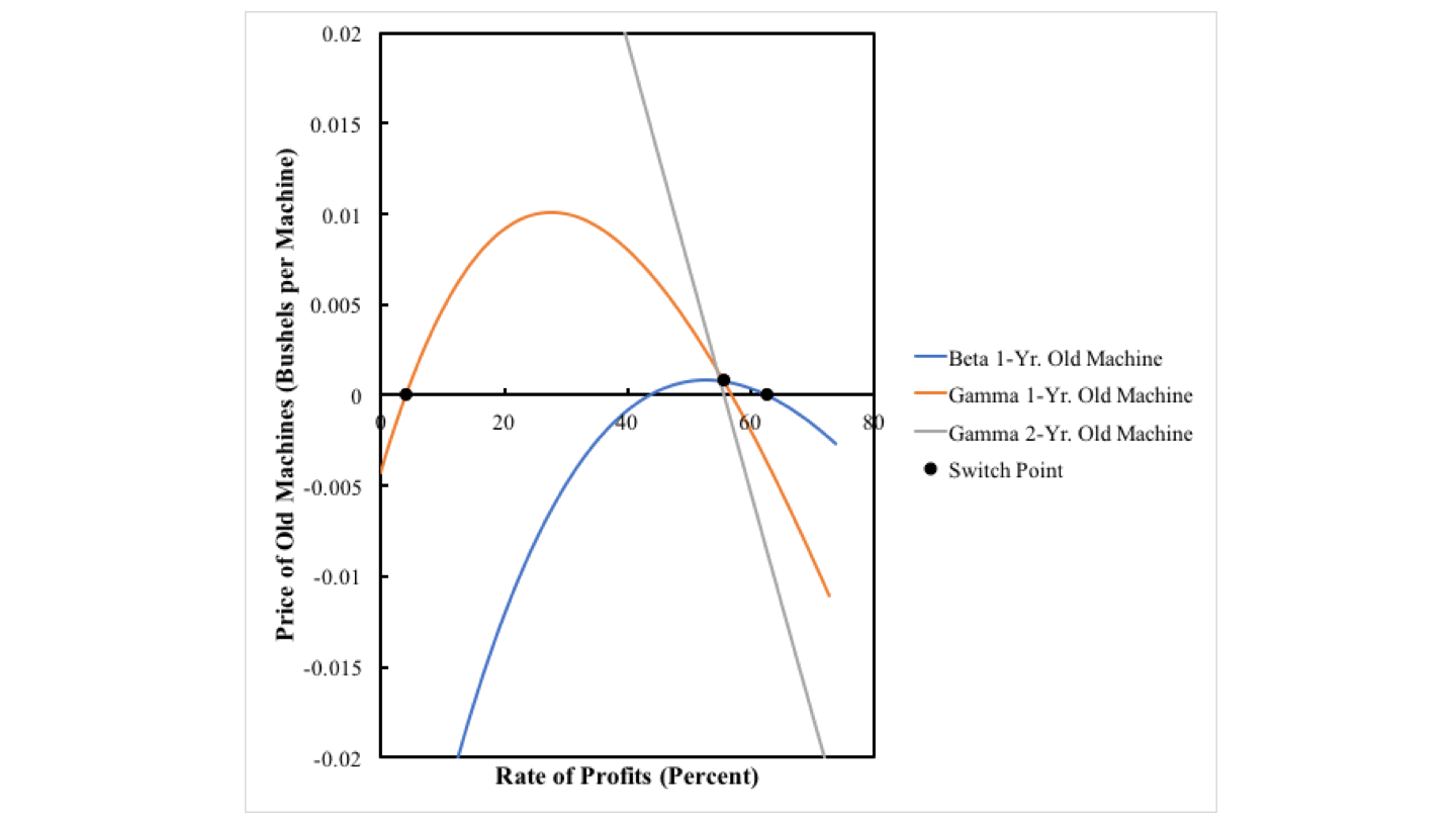
An aspect of the choice of technique can be seen by looking at prices. Figure 3 shows the price of new machines. For all techniques, the price of a new machine is positive for any feasible distribution. At a switch point, the price of a new machine is the same for both techniques that are cost-minimizing. Figure 4 shows how the price of old machines varies with the rate of profits. If a technique is cost-minimizing, the prices of old machines produced by that technique are non-negative at that rate of profits. At a switch point, the price of at least one produced old machine is zero. Baldone's article goes into much detail about prices of machines and truncation.

Figure 3: The Price of a New Machine

The price of an old machine is zero for a technique in which that machine is not produced. Figure 4 shows the prices of only those old machines that are produced in the corresponding technique. In an analysis of the choice of technique with fixed capital, if the price of an old machine is negative at a given rate of profits, the cost minimizing technique must have the economic life of machine must be truncated. Consider, for example, rates of profits less than approximately 4 percent or greater than approximately 63 percent. The price of a one-year old machine under the Beta technique is negative. The prices of one-year old and two-year old machines under the Gamma technique are both negative. Thus, neither can be cost-minimizing. The Alpha technique must be cost-minimizing in these ranges of the rates of profits.

Figure 4: The Price of Old Machines in the Baldone Example

4.0 A Time Path

I now take a first step in generalizing Baldone's capitalism. The rate of decrease of coefficients of production happens to be ten percent in both the machine and corn sectors. Figure 5 shows how the wage frontier varies with time under these assumptions. The maximum rate of profits and the rate of profits at switch points are plotted against time.

Figure 5: Variation in the Wage Frontier with Time

Here, the economy is not viable at the initial time. There must be some sort of low-productivity, backstop technology that was previously used. Figure 5 partitions time into six regions, and Figure 6 enlarges transient regions. Baldone's example is in Region 9.

Figure 6: An Enlargement of the Variation in the Wage Frontier

5.0 A Partition of the Parameter Space

I now let the rates of decrease in coefficients of production differ between the machine and corn sector. Figure 7 graphs the resulting two-dimensional space and how it is partitioned by fluke switch points, which I call patterns. I only label one partition in Figure 7. For the partition between Region 0 and Region 1, the maximum rate of profits for the Alpha technique is zero, and the maximum rate of profits is negative for the Beta and Gamma techniques.

Figure 7: A Two-Dimensional Pattern Diagram

I look at two enlargements of parts ot the space in Figure 7 to get a somewhat more visually obvious understanding of what is going on here. Figure 8 is a blow-up of the middle left of Figure 7, and Figure 1 is a blow-up towards the middle right of Figure 7. I suppose I should say something more about this graph, but I will content myself with Table 3 and one observation. Consider the intersection of the boundaries between Regions 1 and 2, between 2 and 6, between 6 and 7, and between 7 and 1. This point is an intersection of three patterns over the wage axis with a three-technique pattern. I want to claim this intersection is generic, in some sense. I suppose precisely specifying in what sense would be publishable but maybe is beyond me.

Figure 8: An Enlargement of the Parameter Space

Table 3: Results

Region	Technique	Summary
0	None	Not viable.
1	Alpha	No switch points.
2	Beta, Alpha	The switch point exhibits negative real Wicksell effects. A smaller rate of profits is associated with a longer economic life of a machine.
3	Beta	No switch points.
4	Gamma, Beta	The switch point exhibits negative real Wicksell effects. A smaller rate of profits is associated with a longer economic life of a machine.
5	Gamma	No switch points.
6	Gamma, Beta, Alpha	Switch points exhibit negative real Wicksell effects. A smaller rate of profits is associated with a longer economic life of a machine.
7	Gamma, Alpha	The switch point exhibits negative real Wicksell effects. A smaller rate of profits is associated with a longer economic life of a machine.
8	Alpha, Gamma, Alpha	The switch point at the higher rate of profits exhibits positive real Wicksell effects. Reswitching of techniques and recurrence of truncation.
9	Alpha, Gamma, Beta, Alpha	The switch point between Beta and Alpha exhibits positive real Wicksell effects. Recurrence of techniques and of truncation.
10	Alpha, Gamma, Beta	Switch points exhibit negative real Wicksell effects. A smaller rate of profits is associated with a non-monotonic variation in the economic life of machine.
11	Alpha, Gamma	The switch point exhibits negative real Wicksell effects. A smaller rate of profits is associated with a shorter economic life of a machine.

6.0 Non-Monotonic Variation of the Economic Life of a Machine with the Rate of Profits

I might as well illustrate the wage frontier (Figure 9) in Region 10. From low to high wages (that is, high to low rates of profits) the cost-minimizing technique ranges from Beta through Gamma to Alpha. In a stationary state, the machine is run for two years at maximum rate of profits. At a middling rate of profits, its economic life is increased to three years. At an even lower rate, its economic life jumps down to one year. Around both switch points, corn produced per person-year is higher at the lower rate of profits. In some sense, the technique adopted at the lower rate of profits is more capital-intensive, despite the non-monotonic variation in the economic life of the machine. The switch point between Beta and Gamma is consistent with Austrian claims, but the switch point between Gamma and Alpha is a logical disproof of their capital theory.

Figure 9: The Wage Frontier in Region 10

For completeness, Figure 10 plots the prices of produced old machines by technique. For a rate of profits below approximately 10.7 percent, the price of a one-year old machine is negative for both the Beta and Gamma techniques. Thus, neither is cost-minimizing in this range; the Alpha technique is. Between approximately 10.7 and 110 percent, the prices of both one-year old and two-year old machines is positive under the Gamma technique. It is not cost-minimizing to truncate the machine to one or two years in this range. For even larger feasible rates of profits, the price of a two-year old machine is negative under the Gamma technique, and the price of a one-year old machine is positive under the Beta technique. In this range, it is cost-minimizing to operate the machine for two years.

Figure 10: Prices of Old Machines in Region 10

7.0 Conclusion

My methodology for generalizing Baldone's example leads to some complicated graphs. I find a couple of new phenomena that I have not seen in other examples of fixed capital. I think of Region 0, in which no specificed technique is viable. More interesting to me is Region 10, in which the economic life of a machine varies non-monotonically with the rate of profits, without either recurrence of techniques or cost-minimizing.

Reference

• Salvatore Baldone. 1974. Il capitale fisso nello schema teorico di Piero Sraffa. Studi Economici XXIV(1): 45-106. Translated in Pasinetti (1980).

An Extension Of An Example From Salvatore Baldone

Figure 1: A Pattern Diagram, Enlarged

1.0 Introduction

This post looks at and generalizes an example of the recurrence of techniques by Salvatore Barone. It is an example with fixed capital illustrating the recurrence of the period of truncation. In the generalization, I find what I call patterns over the axis for the rate of profits, a patern over the wage axis, a three-technique pattern, and a reswitching pattern.

Barone's example demonstrates that around a switch point, a lower rate of profits can be associated with both an increase and a decrease in the economic life of a machine and an increased life of a machine can be associated with both an increase and a decrease in the capital-intensity of a technique. From other examples, I know the variability in the direction of the period of truncation with the rate of profits, the (non) relationship of the economic life of a machine with output per worker, and the jump (from one years to three) in the economic life of a machine with an infinitesimal variation in the rate of profits are independent of reswitching and capital-reversing.

So much for the Austrian theory of capital.

2.0 Technology

The available technology consists of the four processes in Tables 1 and 2. Each process exhibits constant returns to scale (CRS) and takes a year to complete. In the first process, labor and corn are used to make a machine, which, I suppose, I could have called a tractor. In the remaining three processes, labor, corn, and the machine are used to make corn. In each of the first two of these three processes, a machine one year older than it was as an input is jointly produced with corn. Corn is circulating capital and the machine is fixed capital.

Table 1: Inputs for The Technology

Input	Process
	(I)	(II)	(III)	(IV)
Labor	a0, 1	a0, 2	a0, 3	a0, 4
Corn	a1,1	a1,2	a1,3	a1, 4
New Machines	0	1	0	0
1-Year Old Machines	0	0	1	0
2-Year Old Machines	0	0	0	1

Table 2: Outputs for The Technology

Output	Process
	(I)	(II)	(III)	(IV)
Corn	0	1	1	1
New Machines	1	0	0	0
1-Year Old Machines	0	1	0	0
2-Year Old Machines	0	0	1	0

I assume that an old machine can be costlessly disposed of before its technical life. Thus, there are three techniques that can arise in a stationary state. In the Alpha technique, the machine is junked after being used one year; only the first two processes are operated. In Beta, the machine is junked after two years. In Gamma, the machine is operated for its full technical life and all four processes are operated.

I conclude this section by specifying parameters for the coeffients of production:

a_{0, 1} = (2/5) e^{1 - t/10}

a_{0, 2} = (1/5) e^{1 - t/10}

a_{0, 3} = (3/5) e^{1 - t/10}

a_{0, 4} = (2/5) e^{1 - t/10}

a_{1, 1} = (1/10) e^{1 - t/10}

a_{1, 2} = (2/5) e^{1 - t/10}

a_{1, 3} = 0.578 e^{1 - t/10}

a_{1, 4} = (3/5) e^{1 - t/10}

Barone's example arises when t = 10. The exponential decay in these coefficients is a description of technical progress as exogeneous.

3.0 Prices of Production

I now want to consider prices of production, given the technology at a point of time, specifically for Baldone's example. I take corn as numeraire. For a given technique, each operated process provides an equation. I take labor as advanced and assume wages are paid out of the end of the year. Given the rate of profits, one can then solve for the wage and the prices of a new machine, a one-year old machine, and a two-year old machine.

Figure 2 plots the wage curves for the three techniques. (By the way, Baldone has a transcription error in at least one of his equations. I was able to replicate his tables with this error corrected.) The cost-minimizing techniques are noted, even though which is on the outer frontier is not always easily visible.

Figure 2: The Wage Frontier in Baldones Example

Figure 3 shows the price of a new machine. At a switch point point, prices are identical for the techniques whose wage curves intersect at that switch point. For example, a rate of profits of approximately 4 percent, the price of a new machine for the Alpha and the Gamma technique is the same.

Figure 3: The Price of a New Machine

Figure 4 is finally an example which is visually obvious. The price of an old machine is zero for a technique in which that machine is not produced. Figure 4 shows the prices of only those old machines that are produced in the corresponding technique. In an analysis of the choice of technique with fixed capital, if the price of an old machine is negative at a given rate of profits, the cost minimizing technique must have the economic life of machine must be truncated.

Figure 4: The Price of Old Machines

Consider, for example, rates of profits less than approximately 4 percent or greater than approximately 63 percent. The price of a one-year old machine under the Beta technique is negative. The prices of one-year old and two-year old machines under the Gamma technique are both negative. Thus, neither can be cost-minimizing. The Alpha technique must be cost-minimizing in these ranges of the rates of profits.

At a rate of profits of approximately 56 percent, the price of a one-year old is positive and the same for the Beta and Gamma techniques, and the price of a two-year old machine is zero under the Gamma technique. This is a switch point for the Beta and the Gamma technique. The price of a two-year old machine is negative under the Gamma technique for any rate of profits greater than this. The Gamma technique cannot be cost-minimizing between 56 and 63 percent. Since the price of a new machine and a one-year old machine is positive, in this range, under the Beta technique, it is not cost-minizing to truncate the machine to an economic life of one year. By the same logic, it is not cost-minimizing to truncate the machine at all for rates of profits between 4 percent and 56 percent.

The analysis of the choice of techniques based on prices yields the same conclusions as an analysis based on the construction as the outer wage frontier. Table 3 summarizes characteristics of the Baldone example. The switch point at approximately 56% is the only one of the three that is not 'perverse'. Around this switch point, a lower rate of profits is associated with an increase in the economic life of the machine, a greater capital-intensity, and more output per worker.

Table 3: Summary of Barone Example

0 ≤ r ≤ 4.066%	Alpha cost minimizing.
r ≈ 4.066%	Lower rate of profits associated with a decrease in the economic life of the machine, from three years to one year. Consumption per worker increased.
4.066% ≤ r ≤ 55.656%	Gamma cost-minimizing.
r ≈ 55.656%	Lower rate of profits associated with an increase in the economic life of the machine, from two to three years. Consumption per worker increased.
55.656% ≤ r ≤ 62.732%	Beta cost-minimizing.
r ≈ 62.732%	Lower rate of profits associated with an increase in the economic life of the machine, from one to two years. Consumption per worker decreased.
62.732% ≤ r ≤ 74.166%	Alpha cost minimizing.

4.0 An Extension for Structural Dynamics

I now introduce structural dynamics. I let all coefficients of production for inputs of labor and corn decrease exponentially, at a rate of 10%. Figure 5 illustrates how the variation of the cost-minimizing technique with the rate of profits changes with technical progress. Here, the economy is not viable at the initial time. There must be some sort of low-productivity, backstop technology that was previously used. Figure 5 partitions time into six regions, and Figure 1, at the top of this post enlarges transient regions. Baldone's example is in Region 3.

Figure 5: A Pattern Diagram

5.0 Conclusion

I suppose I should figure out a complete characterization of all six regions, not just Region 3. I now have more examples with fixed capital for my approach to structural economic dynamics than can be comfortably be described in a paper of reasonable length.

I am finding that the analysis of so-called 'paradoxes' in models of the prices of production with fixed capital is an important extension of the Cambridge Capital Controversy. A thorough understanding of the 13-page Chapter X in Sraffa's book only became available in English after mainstream economists had commenced on ignoring certain results.

References

• Salvatore Baldone. 1974. Il capitale fisso nello schema teorico di Piero Sraffa. Studi Economici XXIV(1): 45-106. Translated in Pasinetti (1980).

Political Novels?

I would like suggestions to add to this list:

• Benjamin Disraeli, Coningsby or the New Generation.
• Anthony Trollope, The Way We Live Now.
• Allen Drury, Advise and Consent: A Novel of Washington Politics.
• John Ehrlichman, The Company.
• Anonymous (Joel Klein) Primary Colors: A Novel of Politics.

This is not for Christmas, but some of my personal reading. I am aware that Coningsby is the first of a trilogy, that Advise and Consent is the first of a series, and that Primary Colors has a sequel. Ehrlichman's novel did not make a lasting impression on me. As usual, I find it hard to define what I think groups these together.

Disraeli writing his novels in the midst of trying to climb the greasy pole is hard to fathom:

"The Duke talks to me of Conservative principles; but he does not inform me what they are. I observe indeed a party in the State whose rule it is to consent to no change, until it is clamorously called for, and then instantly to yield; but those are Concessionary, not Conservative principles. This party treats institutions as we do our pheasants, they preserve only to destroy them. But is there a statesman among these Conservatives who offers us a dogma for a guide, or defines any great political truth which we should aspire to establish? It seems to me a barren thing, this Conservatism, an unhappy cross-breed; the mule of politics that engenders nothing." -- Disraeli

Triple Switching and Fluke Switch Points

Figure 1: A Pattern Diagram with Triple Switching

In demonstrating the lack of foundation for claims of the Austrian school about the supposed relationships between a greater supply of capital, a consequent lower rate of profits, and a longer period of production, I have so far only presented examples in which the economic life of an existing machine can be extended or truncated. Schefold (1980: 170) interprets a more roundabout technique as one in which a long-lived machine is used to produce a finished good that previously was produced directly without the aid of fixed capital or, at least, with a different and inferior machine. The example in this post extends Schefold's illustration of the difficulty in sustaining the Austrian claim.

I am disappointed that in briefly exploring the parameter space specified by coefficients of production, I was unable to find an example in which wages curves on the frontier were easily distinguishable by the eye. I did like that Figure 1 came out one way I knew could bring about triple switching.

The second, third, and fourth processes in the technology (Tables 1 and 2) constitute the corn sector. In Process II, corn is produced from inputs of labor and corn, without fixed capital. The Alpha technique (Table 3) consists of Process II alone. A machine sector, composed of Process I, exists in the Beta and Gamma techniques. The technical life of the machine is two years. The machine is truncated to one year in the Beta technique

Table 1: Inputs for The Technology

Input	Process
	(I)	(II)	(III)	(IV)
Labor	a0,1	a0,2	a0,3	a0,4
Corn	a1,1	a1,2	a1,3	a1,4
New Machines	0	0	1	0
Old Machines	0	0	0	1

Table 2: Outputs for The Technology

Output	Process
	(I)	(II)	(III)	(IV)
Corn	0	1	b1,3 = 1/2	b1,4 = 1/2
New Machines	1	0	0	0
Old Machines	0	0	1	0

Table 3: Techniques

Techniques	Processes
Alpha	(II)
Beta	(I), (III)
Gamma	(I), (III), (IV)

Suppose the coefficients of production for inputs of labor and circulating capital decrease ten percent per year. Figure 1 shows the variation in the choice of technique for a specific configuration of coefficients of production. Schefold's example of triple switching occurs at t = 10. Figure 2 graphs the wage frontier here, in which the wage curves for the Alpha and Gamma techniques are difficult for the eye to distinguish. Figure 3 shows extra profits in operating the second process at Gamma prices. Triple switching is more apparent here.

Figure 2: Wage Frontier for Triple Switching

Figure 3: Extra Profits at Gamma Prices

With this specification of parameters and technical progress, the non-roundabout process Alpha eventually replaces the roundabout process Gamma, whatever the distribution of income. Triple switching appears in the middle of the three transient regions. The patterns of switch points illustrate one manner in which triple-switching can appear. If the pattern over the wage axis were to arise before the second reswitching pattern, the region in which triple-switching occurs would be followed by a region with double switching. With more techniques, one of the switch points could be replaced on the frontier in a three-technique pattern, instead of eventually vanishing over an axis. At any rate, this example continues to illustrate how combinations of patterns of switch points can illuminate the effects of technical change.

In Regions 2, 3, and 4, the Alpha technique, in which corn is produced without the use of a machine, is cost-minimizing at the highest rate of profits, where the wage is zero. Around the only switch point in each of Regions 2 and 4, a lower rate of profits is indeed associated with a more roundabout technique, and the more roundabout technique has a higher level of consumption per person-year in a stationary state. The Austrian claim is also illustrated at the lowest and highest switch point in Region 2. But it is invalidated for the middle switch point. Around this switch point, a lower rate of profits is associated with the replacement of a roundabout technique by the direct production of the consumer commodity.

This numerical example re-iterates that no necessary connection exists between employing or lengthening the economic life of a machine and an increase in the use of 'capital'. Bohm-Bawerk (1959) was incorrect not merely because of the difficulty of defining a quantitative measure of the average period of production. His intuition, and not just his, on how prices work was itself incorrect.

A Three-Technique Pattern Over The Wage Axis

Figure 1: Wage Frontier for a Fixed Capital Example

This post presents a perturbation of parameters in a 'one good' model of fixed capital. The coefficients of production differ from those in this reswitching example. But the model has the same structure.

Consider a one-commodity economy in which labor and widgets are used to produce new widgets, the only consumption good. (The use of the term 'widget' to designate the single produced commodity emphasizes how unrealistic this model is.) New widgets last several years when used in producing widgets. In this particular answer to Steedman's homework assignment, they last three years. And their efficiency can vary throughout their technical lifetime. Accordingly, Tables 1 and 2 specify the coefficients of production for three processes.

Table 1: Inputs for The Technology

Input	Process
	(I)	(II)	(III)
Labor	a0,1	a0,2	a0,3
New Widgets	1	0	0
One-Year Old Widgets	0	1	0
Two-Year Old Widgets	0	0	1

Table 2: Outputs for The Technology

Output	Process
	(I)	(II)	(III)
New Widgets	b1,1	b1,2	b1,3
One-Year Old Widgets	1	0	0
Two-Year Old Widgets	0	1	0

Firms are not required to operate all three processes. They can truncate the use of widgets after one or two years. The choice of technique in this model is equivalent to the choice of the economic life of a widget. In the Alpha technique, the widget is operated for one year; in the Beta technique, it is operated for two years; and in the Gamma technique, it is operated for the full three years.

The wage frontier is the outer envelope of all wage curves. In models of circulating and fixed capital without superimposed joint production, the cost-minimizing technique, at a given rate of profits, is the technique which contributes its wage curve to the frontier at that rate. The Gamma technique is cost-minimizing in Figure 1 for all feasible rates of profits. Wage curves, when on the frontier, are declining functions of the rate of profits. At a switch point, more than one technique is cost-minimizing. At a rate of profits of zero in Figure 1, the Alpha, Beta, and Gamma techniques are all cost-minimizing.

The single switch point in Figure 1 is a fluke case several times over. It is the intersection of three wage curves, not two. And the switch point is on the wage axis, occurring for a rate of profits of zero. These properties are destroyed by any variation in certain coefficients of production. Figure 2 illustrates variations in b_1,2 and b_1,3. (The numbering of regions are consistent with this post.) The location in parameter space for fluke switch points, which I call patterns of switch points, is shown. Consider parameters in Region 4, and suppose b_1,2 is increased. Eventually, a fluke case will arise in which the switch point between the Alpha and Beta technique is on the wage axis. When b_1,2 > 10, this switch point will no longer occur for a non-negative rate of profits. It will only be cost-minimizing to run widgets for two or three years, depending on distribution. On the other hand, consider an increase in b_1,3. The switch points between Alpha and Beta and between Beta and Gamma will eventually coincide, in a single switch point at a positive rate of profits. With any further increase in this parameter, it is no longer cost minimizing to run widgets for two years, whatever the distribution of income.

Figure 2: Selected Regions in Parameter Space

Tables 3 and 4 summarize the choice of technique in each region in Figure 2. Negative real Wicksell effects occur at all switch points in the four regions in Figure 2. According to traditional Austrian and marginalist dogma, one might expect an increase in capital intensity to go along with a longer economic life of a widget. This idea is proven to be untrue in Regions 1, 4, and 5. Is the jump over an economic life of two years in Region 1 surprising? Adjacent techniques on the wage frontier need not be near in a parameter space formed by coefficients of production. Continuity in the wage frontier does not imply continuous variation in coefficients of production. In this case, the three-technique pattern of switch points illustrates how managers of firms come to eliminate the choice of the Beta technique.

Table 3: Variation in the Choice of Technique

1	0 ≤ r ≤ r1	Widgets operated for one year
	r1 ≤ r ≤ rγ	Widgets operated for three years
3	0 ≤ r ≤ rγ	Widgets operated for three years
4	0 ≤ r ≤ r1	Widgets operated for one year
	r1 ≤ r ≤ r2	Widgets operated for two years
	r2 ≤ r ≤ rγ	Widgets operated for three years
5	0 ≤ r ≤ r1	Widgets operated for two years
	r1 ≤ r ≤ rγ	Widgets operated for three years

Table 4: Summary of Local Structural Changes

1	A larger rate of profits is associated with a longer economic life of a widget.
3	No switch points.
4	A larger rate of profits is associated with a longer economic life of a widget.
5	A larger rate of profits is associated with a longer economic life of a widget.

This structure in a two-dimensional parameter space is generic, in some sense. Three partitions of patterns over the wage axis intersect in the start of a ray that is a partition for a three-technique pattern. A corresponding structure exists for patterns over the axis for the rate of profits.