|
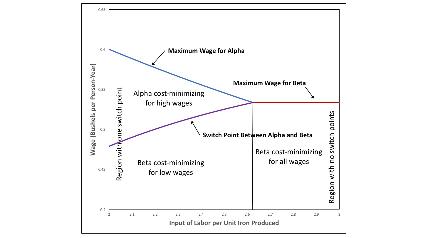
| Figure 1: Bifurcation Diagram |
This post continues a series investigating structural economic dynamics. I think most of those who understand prices of production - say, after working through Kurz and Salvadori (1995) - understand that technical innovation can change the appearance of the wage frontier. (The wage frontier is also called the wage-rate of profits frontier and the factor-price frontier.) Changes in coefficients of production can create or destroy a reswitching example. But, as far as I know, nobody has systematically explored how this happens in theory.
I claim that when switch points appear on or disappear off of the wage frontier, these bifurcations follow a few normal forms. I have been describing each normal form as a story of a coefficient of production being reduced by technical innovation. I further claim that, in some sense, the order of changes along the wage frontier is not specified. One can find an example with a decreasing coefficient of production in which the order is the opposite of some other example of technical innovation with the same normal form.
This post is one of a series providing the proof that order does not matter. The example in this post relates to this previous example.
2.0 TechnologyThe example in this post is one of an economy in which four commodities can be produced. These commodities are called iron, steel, copper, and corn. The managers of firms know (Table 1) of one process for producing each of the first three commodities. These processes exhibit Constant Returns to Scale. Each column specifies the inputs required to produce a unit output for the corresponding industry. Variations in the parameter v can result in different switch points appearing on the frontier. Each process requires a year to complete and uses up all of its inputs in that year. There is no fixed capital.
| Input | Industry | ||
| Iron | Steel | Copper | |
| Labor | 1/2 | 1 | 3/2 |
| Iron | 53/180 | 0 | 0 |
| Steel | 0 | v | 0 |
| Copper | 0 | 0 | 1/5 |
| Corn | 0 | 0 | 0 |
Three processes are known for producing corn (Table 2). As usual, these processes exhibit CRS. And each column specifies inputs needed to produce a unit of corn with that process.
| Input | Process | ||
| Alpha | Beta | Gamma | |
| Labor | 1/2 | 1 | 3/2 |
| Iron | 1/3 | 0 | 0 |
| Steel | 0 | 1/4 | 0 |
| Copper | 0 | 0 | 1/5 |
| Corn | 0 | 0 | 0 |
Four techniques are available for producing a net output of a unit of corn. The Alpha technique consists of the iron-producing process and the Alpha corn-producing process. The Beta technique consists of the steel-producing process and the Beta process. The Gamma technique consists of the remaining two processes.
As usual, the choice of technique is based on cost-minimization. Consider prices of production, which are stationary prices that allow the economy to be reproduced. A wage curve, showing a tradeoff between wages and the rate of profits, is associated with each technique. In drawing such a curve, I assume that a bushel corn is the numeraire and that labor is advanced. Wages are paid out of the surplus product at the end of the year. The chosen technique, for, say, a given wage, maximizes the rate of profits. The wage curve for the cost-minizing technique at the given wage lies on the outer frontier formed from all wage curves.
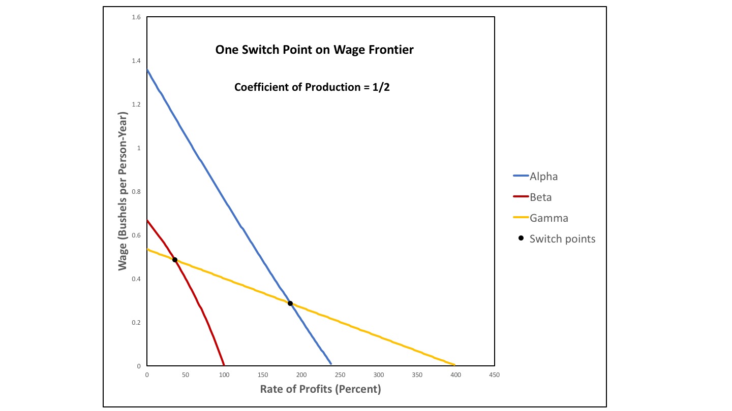
3.0 Technical ProgressFigures 2 through 5 illustrate wage curves for different levels of the coefficient of production denoted v in the table. Figure 2 shows that for a relatively high parameter value, the switch point between the Alpha and Gamma techniques is the only switch point on the outer frontier. For continuously lower parameter values of v, the wage curve moves outward. Figure 3 illustration the bifurcation value, a fluke case in which the wage curves for all three techniques intersect in a single switch point. Other than at the switch point, the wage curve for the Beta technique is not on the frontier. But, for a slightly lower parameter value (Figure 4), the wage curve for the Beta technique, along with switch points between the Alpha and the Beta techniques and between the Beta and Gamma techniques, is on the frontier. The intersection between the wage curves for the Alpha and Gamma techniques is no longer on the frontier. Figure 5 illustrates another bifurcation in the example. The focus of this post is not on this bifurcation, in which a switch point disappears over the axis for the rate of profits.
|
| Figure 2: Wage Curves with High Steel Inputs in Steel Production |

|
| Figure 3: Wage Curves with Medium Steel Inputs in Steel Production |

|
| Figure 4: Wage Curves with Low Steel Inputs in Steel Production |

|
| Figure 5: Wage Curves with Lowest Steel Inputs in Steel Production |
4.0 Discussion
The bifurcation on the right in Figure 1, at the top of this post, is topologically equivalent to the horizontal reflection of the bifurcation on the right in the equivalent figure in this previous post. (On the other hand, the bifurcations on the upper left in both diagrams are the same normal form, in the same order.)
The bifurcation described in this post is a local bifurcation. To characterize this bifurcation, one need only look at small range of rates of profits and coefficients of production around a critical value. Accordingly, then wage curves involved in the bifurcations could intercept any number of times, in some other example of this normal form, at positive rates of profits. Each of the three switch points involved in the bifurcation could have any direction for real Wicksell effects, positive or negative.
The bifurcation, as depicted in this post, replaces one switch point on the wage curve with two switch points. It could be that the switch point disappearing exhibits capital-reversing, and both of the two new switch points appearing also exhibit capital-reversing. But any of five other other combinations are possible.