Tuesday, March 28, 2017

Niall Kishtainy's Pluralist, Popular History Of Economics

This post calls attention to A Little History of Economics, by Niall Kishtainy. Since I only skimmed this in a local bookstore, this post is not a proper review.

Kishtainy's book, in successive chapters, focuses on the lives of specific economists. The concluding chapter asks why one would want to be an economist, a question that is answered, I gather, by the preceding chapters. The book is in the same genre as Robert Heilbroner's The Worldly Philosophers. Since many more economists are covered in a short span, individual chapters are shorter. As I recall, economists (not in this order) covered include:

  • Augustine and Thomas Aquinas
  • Mercantilists
  • Francois Quesnay, Mirabeau, and other Physiocrats
  • Adam Smith
  • David Ricardo
  • Charles Fourier, Robert Owen, and other utopian socialists
  • Thomas Malthus
  • Friedrich List
  • Karl Marx
  • William Stanley and Alfred Marshall
  • German historical school, Austrian school, and the methodenstreit
  • Thorstein Veblen
  • Vladimir Lenin and John Hobson
  • Ludwig von Mises
  • Joan Robinson and Edward Chamberlin
  • John Maynard Keynes
  • Paul Samuelson, J. R. Hicks
  • Friedrich Hayek
  • Arthur Lewis, Paul Rosenstein-Rodan, and Raul Prebisch
  • Robert Solow, Trevor Swan, and Paul Romer
  • Joseph Schumpeter
  • Gary Becker
  • John Von Neumann and John Nash
  • Ken Arrow and Gerard Debreu
  • Fidel Castro, Che Guevara, and Andre Frank
  • James Buchanan
  • Milton Friedman
  • George Akerlof and Joseph Stiglitz
  • Hyman Minsky
  • John Muth, Eugene Fama, and Robert Lucas
  • Ed Prescott and Finn Kyland
  • Behavioral economics
  • Thomas Piketty

Doubtless, if I read the book in detail, I would have objections to specific details. The attempted coverage, however, seems quite impressive. This book extends from before to after most histories. And it covers a wider range of economists than most.

Wednesday, March 22, 2017

Krugman Confused On Trade, Capital Theory

Over on EconSpeak, Bruce Wilder provides some comments on a post. He notes that economists wanting to criticize glib free-market ideology in the public discourse often seem unwilling to discard neoclassical economic theory.

Paul Krugman illustrates how theoretically conservative and neoclassical a liberal economist can be. (I use "liberal" in the sense of contemporary politics in the USA.) I refer to Krugman's post from earlier this week, in which he adapts an analysis from the theory of international trade to consider technological innovation (e.g., robots). Krugman presents a diagram, in which endowments of capital and labor are measured along the two axes. Krugman does not seem to be aware that one cannot, in general, coherently talk about a quantity of capital, prior to and independently of prices. He goes on to talk about "capital-intensive" and "labor-intensive" techniques of production.

I point to my draft paper, "On the loss from trade", to illustrate my point that one cannot meaningfully talk about the endowment of capital.

(I did submit this paper to a journal. A reviewer said it was not original enough. I emphasized that I was illustrating my points in a flow-input, point output model, with a one-way flow from factors of production to consumption goods, not a model of production of commodities by means of commodities. Steedman & Metcalfe (1979) also has a one-way model, albeit with a point-input, point-output model. So the reviewer's comments were fair. Embarrassingly, I cite other papers from that book. Apparently, I had forgotten that paper, if I ever read it. I suppose that, given the chance, I could have distinguished some of my points from those made in Steedman & Metcalfe (1979). Also, I close my model with utility-maximization; if I recall correctly, Steedman leaves such an exercise to the reader in papers in that book.)

Reference
  • Ian Steedman and J. S. Metcalfe (1979). 'On foreign trade'. In Fundamental Issues in Trade Theory (ed. by Ian Steedman).

Saturday, March 18, 2017

Reswitching Only Under Oligopoly

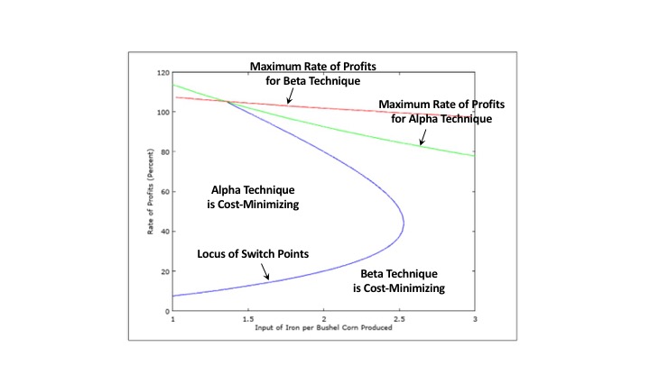
Figure 1: Rates of Profits for Switch Points for Differential Rates of Profits
1.0 Introduction

Suppose one knows the technology available to firms at a given point in time. That is, one knows the techniques among which managers of firms choose. And suppose one finds that reswitching cannot occur under this technology, given prices of production in which the same rate of profits prevails among all industries. But, perhaps, barriers to entry persist. If one analyzes the choice of technique for the given technology, under the assumption that prices of production reflect stable (non-unit) ratios of profits, differing among industries, reswitching may arise for the technology. The numerical example in this post demonstrates this logical possibility.

The numerical example follows a model of oligopoly I have previously outlined. In some sense, the example is symmetrical to the example in this draft paper. That example is of a reswitching example under pure competition, which becomes an example without reswitching and capital reversing, if the ratio of the rates of profits among industries differs enough. The example in this post, on the other hand, has no reswitching or capital reversing under pure competition. But if the ratios of the rates of profits becomes extreme enough, it becomes a reswitching example.

2.0 Technology

The technology for this example resembles many I have explained in past posts. Suppose two commodities, iron and corn, are produced in the example economy. As shown in Table 1, two processes are known for producing iron, and one corn-producing process is known. Each column lists the inputs, in physical units, needed to produce one physical unit of the output for the industry for that column. All processes exhibit Constant Returns to Scale, and all processes require services of inputs over a year to produce output of a single commodity available at the end of the year. This is an example of a model of circulating capital. Nothing remains at the end of the year of the capital goods whose services are used by firms during the production processes.

Table 1: The Technology for a Two-Industry Model
InputIron
Industry
Corn
Industry
Labor1305/4941
Iron1/10229/49411/10
Corn1/403/19762/5

For the economy to be self-reproducing, both iron and corn must be produced each year. Two techniques of production are available. The Alpha technique consists of the first iron-producing process and the lone corn-producing process. The Beta technique consists of the remaining iron-producing process and the corn-producing process.

3.0 Price Equations

The choice of technique is analyzed on the basis of cost-minimization, with prices of production. Suppose the Alpha technique is cost minimizing. Then the following system of equalities and inequalities hold:

[(1/10)p + (1/40)](1 + rs1) + w = p
[(229/494)p + (3/1976)](1 + rs1) + (305/494)wp
[(11/10)p + (2/5)](1 + rs2) + w = 1

where p is the price of a unit of iron, and w is the wage.

The parameters s1 and s2 are given constants, such that rs1 is the rate of profits in iron production and rs2 is the rate of profits in corn production. The quotient s1/s2 is the ratio, in this model, of the rate of profits in iron production to the rate of profits in corn production. Consider the special case:

s1 = s2 = 1

This is the case of free competition, with investors having no preference among industries. In this case, r is the rate of profits. I call r the scale factor for the rate of profits in the general case where s1 and s2 are unequal.

The above system of equations and inequalities embody the assumption that a unit corn is the numeraire. They also show labor as being advanced and wages as paid out of the surplus at the end of the period of production. If the second inequality is an equality, both the Alpha and the Beta techniques are cost-minimizing; this is a switch point. The Alpha technique is the unique cost-minimizing technique if it is a strict inequality. To create a system expressing that the Beta technique is cost-minimizing, the equality and inequality for iron production are interchanged.

4.0 Choice of Technique

The above system can be solved, given s1, s2, and the scale factor for the rate of profits. I record the solution for a couple of special cases, for completeness. Graphs of wage curves and a bifurcation diagram illustrate that stable (non-unitary) ratios of rates of profits can change the dynamics of markets.

4.1 Free Competition

Consider the special case of free competition. The wage curve for the Alpha technique is:

wα = (41 - 38r + r2)/[80(2 + r)]

The price of iron, when the Alpha technique is cost-minimizing, is:

pα = (5 - 3r)/[8(2 + r)]

The wage curve for the Beta technique is:

wβ = (6,327 - 9,802r + 3,631r2)/[20(1,201 + 213r)]

When the Beta technique is cost-minimizing, the price of iron is:

pβ = [5(147 - 97r)]/[2(1,201 + 213r)]

Figure 2 graphs the wage curves for the two techniques, under free competition and a uniform rate of profits among industries. The wage curves intersect at a single switch point, at a rate of profits of, approximately, 8.4%:

rswitch = (1/1,301)[799 - 24 (8261/2)]

The wage curve for the Beta technique is on the outer envelope, of the wage curves, for rates of profits below the switch point. Thus, the Beta technique is cost-minimizing for low rates of profits. The Alpha technique is cost minimizing for feasible rates of profits above the switch point. Around the switch point, a higher rate of profits is associated with the adoption of a less capital-intensive technique. Under free competition, this is not a case of capital-reversing.

Figure 2: Wage Curves for Free Competition

4.2 A Case of Oligopoly

Now, I want to consider a case of oligopoly, in which firms in different industries are able to ensure long-lasting barriers to entry. These barriers manifest themselves with the following parameter values:

s1 = 4/5
s2 = 5/4

In this case, the wage curve for the Alpha technique is:

wα = (4,100 - 4,435r + 100r2)/[40(400 + 259r)]

The price of iron, when the Alpha technique is cost-minimizing, is:

pα = (125 - 96r)/(400 + 259r)

The wage curve for the Beta technique is:

wβ = 8(126,540 - 195,289r + 72,620r2)/[160(24,020 + 9,447r)]

The price of iron, when the Beta technique is cost-minimizing, is:

pβ = 2(3,675 - 3,038r)/(24,020 + 9,447r)

Figure 3 graphs the wage curves for the Alpha and Beta techniques, for the parameter values for this model of oligopoly. This is now an example of reswitching. The Beta technique is cost minimizing at low and high rates of profits. The Alpha technique is cost minimizing at intermediate rates. The switch points are at, approximately, a value of the scale factor for rates of profits of 12.07% and 77.66%, respectively.

Figure 3: Wage Curves for a Case of Oligopoly

4.3 A Range of Ratios of Profit Rates

The above example of oligopoly can be generalized. I restrict myself to the case where the parameters expressing the ratio of rates of profits between industries satisfy:

s2 = 1/s1

One can then consider how the shapes and locations of wage curves and switch points vary with continuous variation in s1/s2. Figure 1, at the top of this post, graphs the wage at switch points for a range of ratios of rates of profits. Since the Beta technique is cost-minimizing, in the graph, at all high feasible wages and low scale factor for the rates of profits, I only graph the maximum wage for the Beta technique. I do not graph the maximum wage for the Alpha technique.

As the ratio of the rate of profits in the iron industry to rate in the corn industry increases towards unity, the model changes from a region in which the Beta technique is dominant to a reswitching example to an example with only a single switch point. As expected, only one switch point exists when the rate of profits is uniform between industries.

5.0 Conclusion

So I have created and worked through an example where:

  • No reswitching or capital-reversing exists under pure competition, with all industries earning the same rate of profits.
  • Reswitching and capital-reversing can arise for oligopoly, with persistent differential rates of profits across industries.

No qualitative difference necessarily exists, in the long period theory of prices, between free competition and imperfections of competition. Doubtless, all sorts of complications of strategic behavior, asymmetric information, and so on are empirically important. But it seems confused to blame the failure of markets to clear or economic instability on such imperfections.

Wednesday, March 15, 2017

Bifurcations in a Reswitching Example

Figure 1: Rates of Profits for Switch Points in One Dimension in Parameter Space
1.0 Introduction

This post presents an example of structural variation in the qualitative behavior of a reswitching example, at different values for selected parameters. I know of few applications of bifurcation analysis to the Cambridge Capital Controversy. Most prominently, I think of Rosser (1983). I suppose I could also point to some of my draft papers. Although not presented this way, one could read Laibman and Nell (1977) as a bifurcation analysis, where the steady state rate of growth is the parameter being varied.

I guess one could read this post as a response to the empirical results in Han and Schefold (2006). Schefold has been developing a theoretical explanation, based on random matrices, of why capital-theoretic paradoxes might be empirically rare. I seem to have stumbled on an explanation of why such paradoxes might arise in practice, and yet might not be observable without more data. To fully address recent results from Schefold, on reswitching and random matrices, one should analyze the spectra of Leontief input-output matrices, which I do not do here.

2.0 Technology

Suppose two commodities, iron and corn, are produced in the economy in the numerical example. As shown in Table 1, two processes are known for producing iron, and one corn-producing process is known. Each column lists the inputs, in physical units, needed to produce one physical unit of the output for the industry for that column. All processes exhibit Constant Returns to Scale, and all processes require services of inputs over a year to produce output of a single commodity available at the end of the year. This is an example of a model of circulating capital. Nothing remains at the end of the year of the capital goods whose services are used by firms during the production processes.

Table 1: The Technology for a Two-Industry Model
InputIron
Industry
Corn
Industry
Labor1305/494a0,2
Iron1/10229/494a1,2
Corn1/403/19762/5

Assume a0,2 is non-negative, and that a1,2 is strictly positive. For the economy to be self-reproducing, both iron and corn must be produced each year. Two techniques of production are available. The Alpha technique consists of the first iron-producing process and the lone corn-producing process. The Beta technique consists of the remaining iron-producing process and the corn-producing process.

3.0 Choice of Technique

Managers of firms choose the technique to adopt based on cost-minimization. I take a bushel of corn as the numeraire. Assume that labor is advanced, and that wages are paid out of the surplus at the end of the year. For this post, I do not bother setting out equations for prices of production; I have done that many times in the past.

3.1 Reswitching for one Set of Parameter Values

Figure 2 illustrates that this is a reswitching example. This figure is drawn for the following values of the labor coefficient in the process for producing corn:

a0,2 = 1

The coefficient of production for iron in corn-production, in drawing Figure 2, is set to the following value:

a1,2 = 2

The economy exhibits capital-reversing around the switch point at an 80% rate of profits.

Figure 2: Wage-Rate of Profits Curves

3.2 Bifurcations with Variations in a Labor Coefficient

Wage-rate of profits curves are drawn for given coefficients of production. And they will be moved elsewhere for different levels of coefficients of production. Consequently, the existence and location of switch points differ, depending on the values for coefficients of production.

Accordingly, suppose all coefficients of production, except a0,2, are as in the above reswitching example. Consider values of the labor coefficient for corn-production ranging from zero to three. The labor coefficient is plotted along the abscissa in Figure 3. The points on the blue locus in the figure show the rate of profits for the switch points, as a correspondence for the labor coefficient. The maximum rates of profits for the Alpha and Beta techniques are also graphed.

Figure 3: Rates of Profits for Switch Points as One Labor Coefficient Decreases

Figure 3 shows a structural change in the example. Up to a value of a0,2 of approximately 2.74, this is a reswitching example. For parameter values strictly greater than that, no switch points exist. The maximum rates of profits for the two techniques are constant in Figure 3. The maximum rates of profits are found for a wage of zero, and they do not vary with the labor coefficient. In some sense, only the maximum rate of profits for the Beta technique is relevant in the figure.

3.3 Bifurcations with Variations in a Coefficient of Production for Iron

Figure 1, at the top of this post, also shows structural changes. The coefficient of production for iron in corn-production varies in the figure. a1,2 ranges from one to three. The other coefficients of production are as in the reswitching example in Section 3.1 above. And the blue locus shows the rate of profits at switch points.

The example can seen to have structural variations here, also, with three distinct regions for a1,2, with the same qualitative behavior in each region. For a low enough value of the coefficient of production under consideration, only one switch point exists. The model remains a reswitching example for an intermediate range of this parameter. And for values of this coefficient of production strictly greater than approximately 2.53, the Beta technique is cost-minimizing for all feasible wages and rates of profits.

The maximum rates of profits, for the Alpha and Beta techniques, are also graphed in Figure 1.

4.0 A Story of Technological Process

Using the above example, one can tell a story of technological progress. Suppose at the start of the story, corn production requires a relatively large input of direct labor and iron, per (gross) unit corn produced. Prices of production associated with this technology are such that only one technique is cost-minimizing. For all feasible wages and rates of profits, firms will want to adopt the Beta technique.

Suppose iron production is relatively stagnant, as compared to corn-production. Innovation in the corn industry reduces the labor and iron coefficients defining the single dominant corn-producing process. After some time, either or both coefficients will be reduced enough that the technology for this economy will have become a reswitching example. And around the switch point at the lower wage (and higher rate of profits), a higher wage is associated with the cost-minimizing technique requiring more labor to be hired, in the overall economy, per given bushel of corn produced (net).

But technological innovation continues to proceed apace. At a even lower coefficient of production for the iron input in the corn industry, the structural behavior of the economy changes again. Now a single switch point exists. And the results of the choice of technique around that switch point conforms to outdated neoclassical intuition.

5.0 Conclusion

This example has two properties that I think worth emphasizing.

The choice of technique in the example corresponds to a choice of a production process in the iron industry. As I have told the story, the technology is fixed in iron production. Innovation occurs in corn production. Thus, innovation in one industry can change the dynamics in another industry.

Second, suppose the technology is observed at a single point of time. Suppose the economy is more or less stationary, and that observation is taken at either the start or the end of the above story. Then neither reswitching nor capital reversing will be observed. Yet such phenomena might arise in the future or have arisen in the past.

References

Saturday, March 11, 2017

Here and Elsewhere

  • A commentator informs me that the True Levelers revived some ideas put forth in the Peasants Revolt.
  • Another commentator points me to Naoki Yoshihara's review of Opocher and Steedman's recent book. Yoshihara has a point, but I think the practice of treating inputs and physically identical outputs as different dated commodities is less applicable in partial models, as opposed to full General Equilibrium. Accountants need guidelines that resist easy manipulation in calculating profits and losses.
  • Antonella Palumbo has a post, "Can 'It' Happen Again? Defining the Battlefield for a Theoretical Revolution in Economics", at the Institute for New Economic Thinking. Palumbo argues that a revival of classical economics, without Say's law, can provide an alternative to neoclassical economics. And Keynes' macroeconomics can be usefully be combined with this revival.

Wednesday, March 08, 2017

A Fluke Switch Point

Figure 1: The Choice of Technique in a Model with Four Techniques
1.0 Introduction

I think I may have an original criticism of (a good part of) neoclassical economics. For purposes of this post, I here define the use of continuously differential production functions as an essential element in the neoclassical theory of production. (This is a more restrictive characterization than I usually employ.) Consider this two-sector example, in which coefficients of production in both sectors varies continuously along the wage-rate of profits frontier. It would follow from this post, I guess, that neoclassical theory is a limit, in some sense, of an analysis in which all switch points are flukes.

I have presented many other, often unoriginal, examples with a continuum of techniques:

I have an example with an uncountably infinite number of techniques along the wage-rate of frontier, but discontinuities for (all?) marginal relationships.

2.0 Technology

I want to compare and contrast two models. The technology in the second model is an example in Salvadori and Steedman (1988).

Households consume a single commodity, called "corn", in both models. In both models, two processes are known for producing corn. And these processes require inputs of labor and a capital good to produce corn. All processes exhibit Constant Returns to Scale, and all processes require services of inputs over a year to produce output of a single commodity available at the end of the year. Both models are models of circulating capital. Nothing remains at the end of the year of the capital goods whose services are used by firms during the production processes.

2.1 First Model

The technology for the first model is shown in Table 1. Each column lists the inputs, in physical units, needed to produce one physical unit of the output for the industry for that column. The two processes for producing corn require inputs of distinct capital goods. One corn-producing process requires inputs of labor and iron, and the other requires inputs of labor and tin.

Table 1: The Technology for a Three-Industry Model
InputIron
Industry
Tin
Industry
Corn
Industry
(a)(b)(c)(d)
Labor1212
Iron002/30
Tin0001/2
Corn2/31/200

Two techniques, as shown in Table 2, are available for producing a net output of corn. A choice of a process for producing corn also entails a choice of which capital good is produced. When the processes are each operated on a appropriate scale, the gross output of the process producing the specific capital good exactly replaces the quantity of the capital good used up as an input, summed over both industries operated in the technique.

Table 2: Techniques in a Three-Commodity Model
TechniqueProcesses
Alphaa, c
Betab, d

2.2 Second Model

The technology for the second model is shown in Table 3. Two processes are known for producing corn. Both corn-producing processes require inputs of labor and iron, but in different proportions.

Table 3: The Technology for a Two-Industry Model
InputIron
Industry
Corn
Industry
(a)(b)(c)(d)
Labor1212
Iron002/31/2
Corn2/31/200

Table 4 lists the techniques available in the second model. The first two techniques superficially resemble the two techniques available in the first model. But, in this model, the first process for producing a capital good can be combined, in a technique, with the second corn-producing producing process. This combination of processes is called the Gamma technique. Likewise, the Delta technique combines the second process for producing a capital good with the first corn-producing processes. Nothing like the Gamma and Delta techniques are available in the first model.

Table 4: Techniques in a Two-Commodity Model
TechniqueProcesses
Alphaa, c
Betab, d
Gammaa, d
Deltab, c

3.0 Prices of Production

Suppose the Alpha technique is cost-minimizing. Prices of production, which permit smooth reproduction of the economy, must satisfy the following system of two equations in three unknowns:

(2/3)(1 + r) + wα = pα
(2/3) pα(1 + r) + wα = 1

These equations are based on the assumption that labor is advanced, and wages are paid out of the surplus at the end of the year. The same rate of profits are generated in both industries. A unit quantity of corn is taken as the numeraire.

One of the variables in these equations can be taken as exogenous. The first row in Table 5 specifies the wage and the price of the appropriate capital good, as a function of the rate of profits. The equation in the second column is called the wage-rate of profits curve, also known as the wage curve, for the Alpha technique. Table 5 also shows solutions of the systems of equations for the prices of production for the other three techniques in the second model, above. I have deliberately chosen a notation such that the first two rows can be read as applying to either one of the two models.

Table 5: Wages and Prices by Technique
TechniqueWage CurvePrices
Alphawα = (1 - 2 r)/3pα = 1
Betawβ = (1 - r)/4pβ = 1
Gammawγ = 2(2 - 2r - r2)
/[3(5 + r)]
pγ = 2(7 + 4r)
/[3(5 + r)]
Deltawδ = (2 - 2r - r2)/(7 + 4r)pδ = 3(5 + r)/[2(7 + 4r)]

Figure 1, at the top of this post, graphs all four wage-curves. The wage curves for the Alpha and Beta techniques are straight lines. In the jargon, the processes comprising these techniques exhibit the same organic composition of capital. The wage curves for the Gamma and Delta techniques are not straight lines. All four wage-curves intersect at a single point, (r, w) = (20%, 1/5). (The wage curves for the Gamma and Delta techniques have the same intersection with the axis for the rate of profits.)

3.0 Choice of Technique

The cost-minimizing techniques form the outer envelope of the wage curves. For a given wage, the cost minimizing technique is the technique with the highest wage curve in Figure 1. A switch point is a point on the outer envelope at which more than one technique is cost-minimizing. All four wage curves intersect, in the figure, at the single switch point.

The Beta technique is cost-minimizing for wages to the left of the single switch point. The Alpha technique is cost-minimizing for all feasible wages greater than the wage at the switch point. Managers of firms replace both processes in the Alpha technique at the switch point with both processes in the Beta technique.

This is no problem for the first model above. The adoption of a new process for producing corn requires, if the economy is capable of self-replacement before and after the switch, that the process for producing iron or tin be replaced by the process for producing the other.

But consider the other model. For all processes in the Alpha technique to be replaced at a switch point, the wage curves for all techniques composed of all combinations of processes in the Alpha and Beta techniques. In other words, in the second model, wage curves for all four techniques must intersect at the switch point. The example in the second model is a fluke.

I have previously explained what makes a result a fluke, in the context of the analysis of the choice of technique. Qualitative properties, for generic results, continue to persist for some small variation in model parameters.

Consider a model with a discrete number of switch points. Consider the cost-minimizing techniques on both sides of a switch point. And suppose that same commodities are produced in both techniques, albeit in different proportions. Generically, only one process is replaced at such a switch point. All processes, except for that one, are common in both techniques.

5.0 A Generalization to An Uncountably Infinite Number of Processes in Each Industry

Consider a model with more than one industry, but a finite number. Suppose each industry has available an uncountably infinite number of processes. And, in each industry, the processes available for that industry can be described by a continuously differentiable production function. Here I present a two-commodity example with Cobb-Douglas production functions.

There are no switch points in such a model. The cost-minimizing technique varies continuously along the outer-envelope of wage curves. In fact, the processes in each industry, in the cost-minimizing technique varies continuously. Since there are no switch points at all, there is not a single switch point in which more than one process varies, as a fluke, with the cost-minimizing technique.

Nevertheless, cannot one see such "smooth" production functions as a limiting case? If so, it would be a generalization or extension of a discrete model, in which all switch points are flukes, to a continuum. From the perspective of the analysis of the choice of technique in discrete models, typical neoclassical models are nothing but flukes.

6.0 Conclusions

I actually found my negative conclusion surprising. I have tried to be conscious of the distinction between the structure of the two models in Section 2 above. I think at least some examples I have presented cannot be attacked by the above critique. They are examples of the first, not the second model. I tend to read Samuelson (1962) in the same way, as not sensitive to the critique in this post.

References
  • Neri Salvadori and Ian Steedman (1988). No reswitching? No switching! Cambridge Journal of Economics, V. 12: pp. 481-486.
  • Samuelson, P. A. (1962). Parable and Realism in Capital Theory: The Surrogate Production Function, V. 29, No. 3: pp. 193-206.
  • J. E. Woods 1990. The Production of Commodities: An Introduction to Sraffa, Humanities Press International.

Saturday, March 04, 2017

Bifurcations Of Roots Of A Characteristic Equation

Figure 1: Rates of Profits for Beta Technique

I have previously considered all roots of a polynomial equation for the rate of profits in a model, of the choice of technique, in which each technique is specified by a finite series of dated labor inputs. One root is the traditional rate of profits, but there are uses for the other roots:

  • All roots appear in an equation defining the Net Present Value (NPV) for the technique, given the wage and the rate of profits.
  • All roots can be combined in an accounting identity for the difference between labor commanded and labor embodied, given the wage.
I thought it of interest to know whether these non-traditional roots are real or complex, as they vary with the wage. I am considering multiple roots in an attempt to build on and critique Michael Osborne's approach to multiple interest rate analysis.

I also have considered examples of models of the production of commodities by means of commodities, in which at least one commodity is basic, in the sense of Sraffa. And I have attempted to apply or extend my critique of multiple interest rate analysis to these models. The point of this post is to illustrate possibilities on the complex plane for multiple interest rates in these models.

A technique in models of the production of commodities by means of commodities, as least in the case when all capital is circulating capital, is specified as a vector of labor coefficients and a Leontief input-output matrix. In parallel with my approach to techniques specified by a finite sequence of dated labor inputs, consider wages as being advanced - that is, not paid at the end of the year out of the surplus - in such models. Given the wage and the numeraire, one can construct a square matrix in which each coefficient is the sum of the corresponding coefficient in the Leontief input-output matrix and the quantity of the commodity produced by that industry that is advanced to the workers, per unit output produced. I call this matrix the augmented input-output matrix.

A polynomial equation, called the characteristic equation, is solved to find eigenvalues of the augmented input-output matrix. The power of this polynomial is equal to the number of commodities produced by the technique. The number of roots for the polynomial is therefore equal to the number of commodities. A rate of profits corresponds to each root. Assume the Leontief input-output matrix is a Sraffa matrix and that the wage does not exceed a certain maximum. Under these conditions, the Perron-Frobenius theorem picks out the maximum eigenvalue of the augmented input-output matrix. The corresponding rate of profits is non-negative, and the prices of production of these commodities are positive at the given wage. I was not able to find an application for the other, non-traditional rates of profits.

I present a numerical example in this working paper. This is a three-commodity example with two techniques. Figure 1 graphs the three roots, at different level of wages, for the Beta technique in that example.

In a previous blog post, I extend that example such that managers of firms have a choice of process for producing each of the three commodities. As a consequence, a choice among eight techniques arises. And one can draw a graph like Figure 1 for each technique in that example. Figure 2 shows the corresponding graph for the Delta technique.

Figure 2: Rates of Profits for Delta Technique

In Figures 1 and 2, the rate of profits picked out by the Perron-Frobenius theorem and used to draw the wage-rate of profits curve for the technique lies along the line segment on the real axis on the left in the figure. A lower wage corresponds to a higher traditional rate of profits. Thus, points further to the right on this line segment correspond to a lower wage. A wage of zero leads to the right-most point on this line segment. The highest feasible wage corresponds to left-most point, at a rate of profits of zero, on this segment.

Two non-traditional rates of profits arise for the other two solutions of the characteristic equation. They are plotted to the right on the graphs in Figures 1 and 2. When complex, they are complex conjugates. I thought it of interest that, in Figure 2, they are purely real for two non-overlapping, distinct ranges of feasible levels of the wage.

I draw no practical, applied implications from the non-traditional rates of profits. I just think the graphs are curious.

Thursday, March 02, 2017

Some Obituaries for Kenneth Arrow

Bill Black has one here, emphasizing Arrow's impossibility theorem. The blog, A Fine Theorem, has two of a planned four-part series. The first is on the impossibility theorem. The second is about General Equilibrium. The two planned, I gather, are to be about learning-by-doing and health economics, respectively.

I have written several posts drawing on Arrow's work. This one, on a sophisticated neoclassical response to the Cambridge Capital Controversy, is among my most popular posts.