A Continuous Time System Block Diagram For Nicholas Kaldor

A System Block Diagram For A Business Cycle Model

In this model of business cycles, two state variables, Y(t) and K(t), represent national income and the value of the capital stock, respectively. These state variables are each specified by a differential equation. In the above block diagram, I have adopted a notation from Steve Keen. The triangles in the upper-right and lower right equate the integrals of their inputs, over time, to their outputs. In other words, the following differential equations obtain:

dY/dt = α[I(t) - S(t)]

dK/dt = I(t) - δK(t)

You can compare and contrast this continuous-time representation of a dynamical system with its analogous discrete-time version.

This is a multiplier-accelerator model that allows for the economy to normally be out of equilibrium. An economic interpretation¹ of the model is that entrepreneurs have some sort of common opinion about the level of economic activity they expect in this nation's economy. And they have an opinion about the total value of capital stock that they believe is needed to sustain that activity. When these expectations are realized, this dynamical system is in an equilibrium. The model shows that when the economy has more activity than expected, entrepreneurs tend to increase the capital stock more rapidly, and vice versa for when activity falls below the expected level. This tendency is a non-linear relationship. Maybe, the more extreme the difference between the actual level and the expected level is, the less likely entrepreneurs are to expect the actual level to continue.

Neither interest rates nor prices are modeled here. Such modeling might be justified by the claim that the income effects in the model overwhelm the effects of prices. At any rate, this model does not contain an aggregate production function. Capacity can be operated either above or below the rate that was desired when the capital equipment being evaluated was installed. If the value of the capital stock falls below the expected level, entrepreneurs tend to increase investment, and vice versa for when the value of the capital stock rises above the expected level. (I think of the depreciation of the capital stock shown in the model as an accounting heuristic, not a physical decay.)

I am not putting forth grand empirical claims. To me, this model is of mathematical interest. It illustrates how non-linear economic dynamics can be generated endogenously. A source of continuous external shocks is not needed².

Unlike in the discrete-time case, I do not see how the continuous-time model given here can generate chaos. Trajectories in the two-dimensional state space are smooth, with no gaps. They cannot intersect. So, I think, this continuous-time model can generate cycles, but not strange attractors³. Another difference between discrete-time and continuous-time systems revolves around the details of stability analysis⁴.

Anyways, the graphical specification of the Kaldor model, given in this post, is suitable for numerical exploration in Steve Keen's software, as I understand it.

Footnote

1. As I understand it, mainstream macroeconomists currently reject the rough-and-ready microfoundations I provide here. They insist on formal microfoundations, even though their preferred formal treatments are just nonsense.
2. Some more mainstream economists seem to be willing to make this points in Overlapping Generations (OLG) models. I am willing to explore the mathematics there, despite the absurdity of assuming investment is driven by intertemporal utility-maximization of consumption.
3. The logistic equation is an example of a one-dimensial, discrete-time, chaotic dynamical system. Off-hand, I cannot think of a continuous-time chaotic system with less than three dimensions.
4. In discrete-time systems, one analyzes the stability of a fixed point by analyzing whether the eigenvalues of the system, linearized around the fixed point, are inside or outside the unit circle in the complex plane. In a continuous-time system, one looks to see if the eigenvalues are to the left or the right of the complex axis, if I recall correctly.

A System Block Diagram For Nicholas Kaldor

A System Block Diagram For A Business Cycle Model

I have previously presented a (replication of an) analysis of a discrete-time formalization of Kaldor's Keynesian model of business cycles. The system block diagram, above, is another way of specifying the model. This diagram, I think, helps make certain characteristics of the system more readily apparent:

• The non-linear component of the system, that is, the inverse tangent function, stands out.
• Only two state variables, national income (Y_t) and the value of the capital stock (K_t), need to be specified for this system.
• The ordered pair (Y_t, K_t) = (μ, σμ/δ) is a fixed point of the function specified by this system.

I am not sure about the use of one-step time lags to represent iteration for the Kaldor model. Presumably, Steve Keen has thought about this question for his software.

I think Keynes' General Theory can be read as leading towards systems thinking prior to its development in other disciplines.

Empirical Bifurcation Diagram For Kaldor Model

Figure 1: An Empirically-Constructed Bifurcation Diagram

I thought I would try to summarize what I have learned about the qualitative behavior of Kaldor's business cycle model. (Although I had some preparation, I learned much of the mathematics in this post during this analysis.) Figure 1, above, shows (mostly) bifurcations found empirically, while Figure 2 below shows bifurcations that can be found analytically. The normalized model is specified by four parameters, the speed of adjustment of national income to the difference between aggregate demand and supply, the depreciation rate of capital, the (average and marginal) propensity to save out of income, and the cost of adjusting the capital stock to the desired level. Figures 1 and 2 are drawn for a constant depreciation rate (δ = 1/5) and a constant cost of adjustment (γ = 3/5). The abscissa in the figures represents different levels of the speed of adjustment (α), while the ordinate represents different levels of the propensity to save (σ).

Figure 2: An Analytically-Constructed Bifurcation Diagram

The Kaldor model has two (endogenously determined) state variables, the normalized level of the capital stock (k_t) and the normalized flow of national income (y_t). A bifurcation analysis determines regions in the parameter space in which the flows for the state variables qualitatively differ. A bifurcation is a manifold in the parameter space in which some such qualitative difference arises. The figures above show selected bifurcations, where each bifurcation is represented by a line or curve in the figure. (I do not claim that the bifurcations shown are the complete set of bifurcations that arises, even in the part of the parameter space shown. For example, I ignore homoclinic bifurcations of points along a limit cycle with the (in)stability of a saddle point.)

The horizontal line near the top of Figure 1 is shown near the bottom of Figure 2. This line represents a pitchfork bifurcation. The model has one fixed point (stationary state), at the origin of the state space, above the line. The model has three fixed points below the line, one at the origin, and the other two symmetrically located around the origin in the first and third quadrants. As I understand it, the origin always has saddle-point (in)stability below this line.

The blue curve in Figure 2 arcing upward to the right from the horizontal line is a Neimark-Sacker bifurcation. (The Neimark-Sacker bifurcation is the discrete time analog to the Hopf bifurcation.) To the left of this curve, the fixed point at the origin is stable. The origin loses its stability at the Niemark-Sacker bifurcation, and it throws out a stable limit cycle to the right. A limit cycle corresponds to a business cycle in the modeled economy.

I think that the bifurcations in the region with three fixed points, below the horizontal line representing the pitchfork bifurcation, are more complicated and more difficult to understand. In the lower left of Figure 1, the two symmetrical fixed points not at the origin are stable. One can find each fixed point's basin of attraction in the state space, that is, those values of the state variables such that a trajectory in the state space started with those values converges to the given fixed point. As I understand it the two basins of attraction cover the entire state space in this region of the parameter space.

Figure 1 shows three (hard to distinguish) curves coming down from the horizontal line and curving to the right. All of these curves intersect the horizontal line at the same point. And that point is also the intersection with that horizontal line of the curve above the horizontal line representing the Neimark-Sacker bifurcation I have previously described. (I have no idea how you would formally prove this.)

The lowest of these curves sloping downward to the right represents a bifurcation in which a limit cycle with saddle point stability appears. Along this curve in the parameter space, a region exists in the state space in which trajectories approach the limit cycle, only to ultimately diverge to one of the fixed points away from the origin.

The next higher curve sloping downward to the right in Figure 1 is almost impossible to tell apart from the curve that I have just described. This curve represents a homoclinic bifurcation. The basins of attraction of the fixed points away from the origin no longer combine to cover the state space. At the homoclinic bifurcation, the stable and unstable sets of the origin merge. Between the lower curve and this curve, the limit cycle with saddle-point stability bifurcates to form (at least) two limit cycles, one stable and one unstable. The unstable limit cycle is the boundary of the union of the basins of attraction of the two stable fixed points. Just above this curve, the border of the basins of attraction bifurcates, to form two disjoint unstable limit cycles. The stable limit cycle remains in the state space, enclosing the fixed point at the origin and these unstable limit cycles.

The highest curve sloping downward to the right in Figure 1 is another Neimark-Sacker bifurcation. The fixed points away from the origin lose their stability at this bifurcation. Their basins of attraction disappear. The unstable limit cycles forming the border of each basin of attraction are absorbed into the corresponding limit point. A stable limit cycle remains. So on the right of Figure 1, both above and below the horizontal line, a stable limit cycle exists, even though the number of fixed points varies with the propensity to save.

I was surprised at the diverse and complex behavior that economists have found in the Kaldor model, a model of the business cycle that is nearly three-quarters of a century old.

A Poincaré Return Map

Figure 1: Definition of A Poincaré Return Map

1.0 Introduction

Poincaré return maps are a useful tool for analyzing the local stability of limit cycles of a dynamical system. In this post, I explain how I define such a map for the Kaldor model of business cycles. I use the Poincaré return map to explain both the existence of a certain limit cycle with saddle-point stability and aspects of a sequence of bifurcations in the model. (My analysis of the Kaldor model also includes these two posts.) I have questions both about the rigorous definition of the Poincaré return map for a discrete-time system and about the consistency of my results with those in Agliari et al. (2007).

2.0 The Domain

The domain of the Poincaré return map, as I define it for the Kaldor model, is a line segment in the phase space. The upper left part of Figure 1 illustrates the phase space. The abscissa is the normalized value of the capital stock, and the ordinate is national income. Notice the line segment sloping upward to the right. It starts at the fixed point at the origin, and goes through the fixed point in the first quadrant. The domain for the map, as illustrated, is the line segment starting at this fixed point and continuing the ray from the origin an arbitrary distance upward. The argument of the Poincaré return map is then the distance along this line segment, with a value of zero corresponding to the fixed point.

Aside: The domain of the Poincaré return map can be used to define a split function¹, useful in locating a homoclinic bifurcation of the origin, in the Kaldor model. (See Figure 3 here.) Let

• x^s be the point in the domain of the Poincaré return function for the first crossing of the stable set of the origin with this domain, when the orbits comprising the stable set are followed backward in time.
• x^u be the point in the domain of the Poincaré return function for the first crossing of the unstable set of the origin with this domain, when the orbits comprising the stable set are followed forward in time.

Define:

β = x^u - x^s

β is a function of the parameters of the Kaldor model. This is a split function, and its value is zero when a homoclinic bifurcation of the origin occurs. End of aside.

3.0 Definition of the Value of the Function

The Poincaré return map defines a discrete time dynamical system with one dimension less than the dynamical system, either continuous or discrete time, for which it is defined. The argument defines a point on the line segment in phase space corresponding to the domain of the map. Imagine an orbit in phase space starting at that point. Follow this orbit until, in this case, it crosses the extended line segment, defining the domain, from above. The point of intersection for this first crossing defines the value of the Poincaré return map for the given argument. It is the distance along this line segment from the fixed point in the first quadrant.

Since the Kaldor model is a discrete time dynamical system, an orbit starting on the line segment defining the domain of the map will likely not have a point on this line segment for the first crossing of the domain. This is not a problem for the numerical computation of the map; the computer program can calculate the intersection of the domain with the two points on the orbit straddling the line segment for the domain. I think this calculation of such intersections is the cause of the small wave-like ripples in the plot of the Poincaré return map in Figure 1. This likely failure of the points on an orbit to lie on the line segment defining the domain for a given positive number of crossing does raise a question in my mind about how to rigorously define the Poincaré return map for a discrete time dynamical system. Perhaps the map is only well-defined for a discrete set of parameter and argument values. I also wonder if the map will miss interesting orbits in phase space².

A line sloping upward at 45 degrees is plotted in red in Figure 1 along with the Poincaré return map. Intersections of the map with this line are fixed points for the Poincaré return map. A fixed point corresponds to a limit cycle in phase space. The slope of the map at these intersections reflects the stability of the corresponding limit cycle:

• If the Poincaré return map is tangent to the 45^o line, the corresponding limit cycle in phase space has the stability of a saddle-point.
• If the Poincaré return map slopes upward steeper than the 45^o line at the point of intersection, the corresponding limit cycle is unstable.
• If the 45^o line slopes upward steeper than the Poincaré return map at the point of intersection, the corresponding limit cycle is stable.

4.0 A Fold Bifurcation

I ignored my qualms about the definition of the Poincaré return map and proceeded with an analysis of limit cycles in the Kaldor model. Figure 2 shows the location of fixed points of the map for an increasing savings rate and certain specified values of the remaining model parameters. No limit cycles exist for small values of the savings rate. A business cycle with the stability of a saddle point appears at a certain value of the savings rate. This limit cycle bifurcates into a stable and an unstable business cycle for higher values of the savings rate. Thus, Figure 2 is a bifurcation diagram for a fold bifurcation of the dynamical system defined by the Poincaré return map.

Figure 2: A Fold Bifurcation of The Poincaré Return Map

5.0 Questions

It seems to me that the above explains³ how a stable and unstable limit cycle arise in the Kaldor model, for example in Figure 3. Agliari et al. (2007) give a different explanation involving Arnold tongues and homoclinic bifurcations of the points comprising certain low-period orbits in phase space with saddle point stability. They claim that a number of such low-period orbits, with changing stability, appear in a sequence of bifurcations in the Kaldor model⁴. I do not see such orbits in the Poincaré return map for the region of parameter space that I have analyzed here. Figure 2 illustrates a local stability analysis, and homoclinic bifurcations seem to be only apparent in a global analysis. I do not understand how my analysis relates to theirs, albeit Agliari et al. state that much of the complexity that they analyze disappears in a final bifurcation in the sequence they describe.

Figure 3: A Stable and Unstable Limit Cycle in the Kaldor Model

Footnotes

1. Figure 6.4, p. 198, in Section 6.1 of Kuznetsov (1998) illustrates a split function.
2. Figure 4.10, p. 129, in Section 4.6 of Kuznetsov (1998) illustrates points in a low-period stable limit cycle and a saddle cycle alternating in a orbit arising in a Neimark-Sacker bifurcation. It is not clear to me how both orbits would show up in my numerically-calculated plots of the Poincaré return map.
3. Figure 5-13, in Section 5.3 of Kuznetsov (1998) illustrates a fold bifurcation of a Poincaré return map and its connection with limit cycles in phase space.
4. These bifurcations, I guess, are related to a Neimark-Sacker bifurcation of the fixed point at the origin.

References

• Agliari, A.; R. Dieci; and L. Gardini (2007). "Homoclinic Tangles in a Kaldor-Like Business Cycle Mode", Journal of Economic Behavior & Organization. V. 62: 324-347.
• Kuznetsov, Y. A. (1998). Elements of Applied Bifurcation Theory, Second edition. Springer-Verlag.

And I know that soon the sky will split And the planets will shift

Figure 1: A Business Cycle

I have been reporting some results from a bifurcation analysis of a formalization of Kaldor's 1940 model of the business cycle. Figures 1 and 2 illustrate the appearance of a business cycle with saddle-point stability in the Kaldor model. Suppose orbits like this arose in the dynamical system governing the solar system. Then the planets might form out of a nebular cloud. And the planets would whirl around their orbits for, maybe, millions of millenia. But then the planets will move away from their orbits, as the solar system falls apart.

Figure 2: National Output in The Business Cycle

By the way, my evidence for the existence of a limit cycle with saddle-point stability consists of graphical representations like these. I have not yet been able to find a sequence of (presumably 62) points that exactly repeat. Each of these points along such a limit cycle would have a corresponding stable and unstable set. And the possibility arises of these stable and unstable sets intertwining in a complicated fashion away from the limit cycle. The title of Agliari et al.'s paper refers to such homoclinic tangles of the stable and unstable sets of points along a limit cycle with saddle point stability. The title is not referring to a homoclinic bifurcation of a limit point at the origin, albeit they point out that bifurcation also.

References

• Agliari, A.; R. Dieci; and L. Gardini (2007). "Homoclinic Tangles in a Kaldor-Like Business Cycle Model", Journal of Economic Behavior & Organization. V. 62: 324-347.

A Homoclinic Bifurcation

Figure 1: Ascending and Descending

I have been presenting some results from an analysis of formalizations of Kaldor's 1940 model of the business cycle. This post illustrates some possible behaviors qualitatively similar to those already reported in the literature.

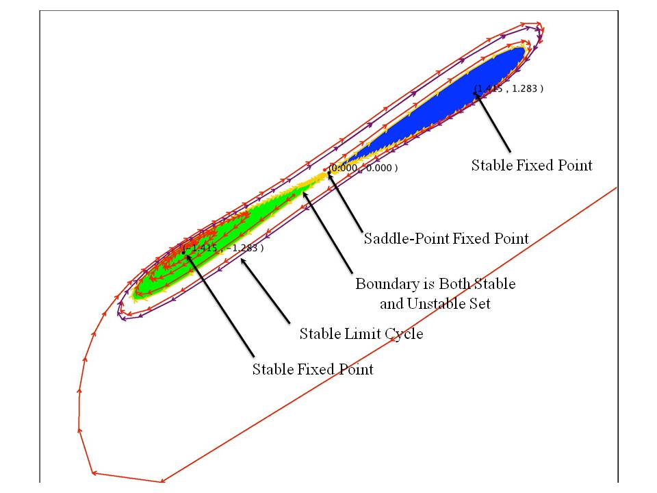
Figures 2, 3, and 4 display some orbits in the (normalized) state space of the Kaldor model, with variations in one parameter determining variations in the topology of these particular phase portraits. In each figure, a movement to the right along the x axis corresponds to an increase in the value of the economy's stock of capital. A movement upward along the y axis corresponds to an increase in the national income. The propensity to save is higher for each figure in the series, but the propensity to save is always small enough that three fixed points exist for the model. In all cases, the middle fixed point has the (in) stability of a saddle point.

Figure 2: Kaldor's Model without a Business Cycle

Figure 3: A Homoclinic Bifurcation in Kaldor's Model

Figure 4: A Business Cycle in Kaldor's Model

A saddle point is such that a ball starting in the direction of the horse's head or tail rolls downward to the center. The bright yellow orbit in each of the three figures represents such a trajectory. The yellow line is known as the stable set of the corresponding fixed point. A ball would have to be balanced just so to achieve such a trajectory on an actual saddle. A ball perturbed from the center of the saddle would tend to roll downward to either side of the horse. The light blue (cyan) orbit in Figures 2 and 4 represent such a trajectory, called the unstable set of the corresponding fixed point.

A bifurcation analysis identifies qualitative changes in the phase portraits for a dynamical system with variations in the system parameters. Several bifurcations exist between Figures 2 and 3, and, I think, two bifurcations arise between Figures 3 and 4. The stable and the unstable sets of the fixed point at the origin, in some sense, have switched roles in the illustrated bifurcations. In Figure 2, the unstable set shown flows from the origin to the other two fixed points. In Figure 4, the stable set flows backwards in time from the origin to the other two fixed points. Of course, some other global behavior is an important difference among these figures. For example, a business cycle does not exist in Figure 2, while Figures 3 and 4 both display a stable business cycle. In the language of dynamical systems, this business cycle is known as a (stable) limit cycle.

The stable and the unstable sets of the origin correspond in Figure 3. Such correspondence of these sets for a given fixed point (or, say, limit cycle) is known as a homoclinic bifurcation. Homoclinic bifurcations are global phenomena and cannot be identified by a merely local stability analysis of the given fixed point. Can you see why one might draw an analogy between a homoclinic bifurcation and the M. C. Escher etching I choose to head this post with?

References

• Agliari, A.; R. Dieci; and L. Gardini (2007). "Homoclinic Tangles in a Kaldor-Like Business Cycle Mode", Journal of Economic Behavior & Organization. V. 62: 324-347.
• Bischi, G. I.; R. Dieci; G. Rodano; and E. Saltari (2001). "Multiple Attractors and Global Bifurcations in a Kaldor-type Business Cycle Model", Journal of Evolutionary Economics. V. 11: 257-554.

A Chaotic Business Cycle

Figure 1: A Chaotic Attractor in Kaldor's Model of the Business Cycle

I might as well post another interim result from my analyses of formalizations of Kaldor's business cycle model. (Today, Noah Smith also posts about chaotic dynamics.) Figure 1 is based on Figure 3 in a 2006 paper from Orlando Gomes. Table 1 shows the parameter values for the model used to generate this figure. For these parameters, Kaldor's model has one attractor, and that attractor is chaotic. The figure shows 1,000,000 (presumably non-transient) points on a single orbit. Although maybe not apparent from the figure, the orbit rotates around the origin in a clockwise direction.

Table 1: Values of Model Parameters

Parameter	Value
Speed of adjustment (α)	12
Depreciation rate (δ)	0.2
Propensity to Save (σ)	0.13
Expected level of output (μ)	200
Cost to adjust capital stock (γ)	0.6

In this model, for these parameters, every business cycle looks somewhat different from the previous one. Yet the model is deterministic. Variations among business cycles, in this model, are not coming from a source of random shocks. Furthermore, the figure shows a fractal structure across business cycles that may not be apparent to agents in the model living through five or ten cycles.

In Figure 1, I've also shown the model's fixed points and indicated their stability. The stability of fixed points in a dynamical system can be analyzed by looking at the eigenvalues of a linear approximation to the system at each fixed point (Figure 2). Methods exist to determine the stability of a fixed point without actually calculating eigenvalues. But the calculation of eigenvalues and eigenvectors is needed to numerically determine the location of the stable and unstable sets at interesting fixed points (albeit I do not show such sets in Figure 1).

Figure 2: Eigenvalues and Stability

References

• Andronov, A. A., E. A. Leontovich, I. I. Gordon, and A. G. Maier (1971). Theory of Bifurcations of Dynamic Systems On a Plane (Translated from Russian), National Aeronautics and Space Administration.
• Gomes, Orlando (2006). "Routes to Chaos in Macroeconomic Theory", Journal of Economic Studies, V. 33, N. 6: 437-468.
• Kuznetsov, Y. A. (1998). Elements of Applied Bifurcation Theory, Second edition. Springer-Verlag.

A Nonergodic Model of the Business Cycle

Figure 1: A Fractal in the Phase Diagram for One Specification of Parameters in the Kaldor Model1

1.0 Introduction

I thought I would try to combine an ability for computers to draw fractals with an economic model that suggests practical conclusions. In this post, I merely duplicate some results in the literature. In a deterministic ergodic process, as I understand it, all trajectories pass through every state in whatever attractor may exist. Hence, the Kaldor model, like some dynamical systems arising in mathematics, is non-ergodic.

2.0 The Model

In 1940, Nicholas Kaldor proposed a model of the business cycle. It can be expressed by four equations². National ouput evolves from the previous period as a response to aggregate demand:

Y_t+1 = Y_t + α(I_t - S_t),

where Y_t is the value of output in year t, I_t is intended investment, and S_t is intended saving. The parameter α represents the speed of adjustment to excess aggregate demand. The evolution of the value of the capital stock depends on investment and depreciation:

K_t+1 = I_t + (1 - δ)K_t,

where δ is the depreciation rate of capital stock. Intended saving is directly proportional to output:

S_t = σY_t,

where σ is the (average and marginal) propensity to save. An investment function³ is the final equation specifying the model:

I_t = σμ + γ(σμ/δ - K_t) + Tan^-1(Y_t - μ),

where μ is the expected level of output, and γ represents the costs of adjusting the capital stock. Along with some restrictions on the values of parameters, the model is now fully specified. The arc tangent function provides a s-shaped non-linear term, such that entrepreneurs increase investment when output exceeds their expectations⁴.

I find it convenient to define new variables normalized around a stationary state:

k_t = K_t - σμ/δ

y_t = Y_t - μ

The model, expressed in terms of normalized capital stocks and normalized output, is:

k_{t + 1} = Tan^-1(y_t) + (1 - δ - γ)k_t

y_{t + 1} = (1 - ασ)y_t + αTan^-1(y_t) - αγk_t

Note that the following is a solution:

For all time t, y_t = k_t = 0.

3.0 Some Results

The above version of the Kaldor model is a discrete-time dynamical system, defined by a map from the two-dimensional real plane (k, y) to the same space. Four⁵ parameters are used to define the map. Questions for the mathematician revolve around describing how the phase portrait for the system varies qualitatively with variations in the parameters. Complex and chaotic behavior can arise in the Kaldor model with appropriate choices of parameter values.

For a small enough speed of adjustment and large enough propensity to save, the dynamics is boring. All trajectories converge to the origin.

As the propensity to save decreases, the system goes through a pitchfork bifurcation, so-called because the bifurcation diagram looks like a pitchfork. The origin loses its stability, and two symmetric fixed points appear. For a small enough speed of adjustment, at least, the two symmetric fixed points exhibit local asymptotic stability. The location of these new fixed points must be found numerically. A fortiori, the computer must be used as an aid to perform a local stability analysis of these points, based on the eigenvalues of the Jacobian matrix.

As the speed of adjustment increases, the boundary between the basins of attraction becomes more complex. Figure 1 shows a case where they are entangled in a fractal-like structure, and the outer perimeter of the colored area is repelling. The limit cycle shown is a short distance outside this repelling boundary.

I have by no means exhausted the dynamics of the Kaldor model. Consider a region in which the origin is the only fixed point, and it is asymptotically stable. As the speed of adjustment increases, the system undergoes a Neimark-Sacker bifurcation, which, I gather, is the discrete-time analog to a Hopf bifurcation. Cycles exist in which the cycle is not a fixed point on the Poincaré return map, but winds around many times before repeating. And if I want my application to explore all these dynamics, I have quite a bit of programming to do. I am curious if I will be able to plot a bifurcation diagram, given that the behavior at the limit depends on the initial value.

4.0 Observations

For the parameter values illustrated in the figures, trajectories have three possible destinations:

• A stable equilibrium with lots of capital and high output.
• Another stable equilibrium with less capital and less output.
• A business cycle.

Furthermore, the boundary between the basins of attraction for the stable limit points is fractal-like. These properties suggest that a random shock to the system can redirect trajectories to a very different final destination.

Although not illustrated above, the model exhibits structural instability. A perturbation of the model parameters can result in different observable behavior, of greater or less complexity.

One general way of conceptualizing business cycles is to see them as the response of a damped linear system to exogenous shocks. Their height and depth depends on the characteristics of the external impulses driving the system. The Kaldor model suggests another possibility. In this model, the properties and extent of business cycles are endogenously determined. Shocks can drive the system from one trajectory to another, but the range of possible behaviors is determined from within the system. It is my impression that the former way of understanding business cycles is dominant among mainstream macroeconomists, while the latter is closer to describing actually existing capitalist economies.

Footnotes

1. Figure 1 is drawn with the parameter values specified in Figure 2(c) in Agliari et al (2007).
2. Kaldor uses a nonlinear savings function and merely specifies the form of the investment function.
3. The specification of investment independent of saving is an essential characteristic of Keynesian models.
4. In this model, expectations are held constant.
5. Notice the expected level of output does not appear in the two equations giving the normalized model.

Selected References

• A. Agliari, R. Dieci, and L. Gardini (2007). Homoclinic Tangles in a Kaldor-like Business Cycle Model. Journal of Economic Behavior & Organization. Vol. 62: 324-347.
• W. W. Chang and D. J. Smyth (1971). The Existence and Persistence of Cycles in a Non-linear Model: Kaldor's 1940 Model Rexamined. Review of Economic Studies. Vol. 38, No. 1: 37-44.
• Richard M. Goodwin (1951). The Nonlinear Accelerator and the Persistence of Business Cycles. Econometrica. Vol. 19, No. 1: 1-17.
• Nicholas Kaldor (1940). A Model of the Trade Cycle. Economic Journal. Vol. 50, No. 197: 78-92.
• Yuri A. Kuznetsov (1998). Elements of Applied Bifurcation Theory, 2nd edition.