Festschrifts for Sraffians

We are on, maybe, the third generations of Sraffians. An annoyance and a delight of publicly taking up a topic is that one must continually read advances, whether large or small, in your topic. I've read some festschrifts over the last several decades:

• Competing Economic Theories: Essays in memory of Giovanni Carvale, edited by Serio Nisticó and Domenico Tosato.
• Value, Distribution and Capital: Essays in honour of Pierangelo Garegnani, edited by Gary Mongiovi and Fabio Petri.
• Economic Theory and Economic Thought: Essays in Honour of Ian Steedman, edited by John Vint, J. Stanley Metcalfe, Heinz D. Kurz, Neri Salvadori, and Paul A. Samuelson.

I'm aware of some I have not read:

• Social Fairness and Economics: Essays in the spirit of Duncan Foley, edited by Lance Taylor, Armon Rezai, and Thomas Michl.
• Keynes, Sraffa and the Criticism of Neoclassical Theory: Essays in honour of Heinz Kurz, edited by Neri Salvadori and Christian Gehrke.
• Classical Political Economy and Modern Theory: Essays in honour of Heinz Kurz, edited by Christian Gehrke, Neri Salvadori, Ian Steedman and Richard Sturn.
• Economic Theory and its History, edited by Guiseppe Freni, Heinz D. Kurz, Andrea Mario Lavezzi, and Rudolfo Signorino. (This apparently is a celebration of Neri Salvadori's work.)
• Production, Distribution and Trade: Essays in honour of Sergio Parrinello, edited by Adriano Birolo, Duncan K. Foley, Heinz D. Kurz, Bertram Schefold and Ian Steedman
• The Evolution of Economic Theory: Essays in honour of Bertram Schefold, edited by Volker Caspari.

This post provides another demonstration that at least one school of heterodox economists looks, from the outside, like any other group of academics with common research interests. I have posted about Post Keynesianism in this respect. Likewise, I once listed textbooks.

A Story Of Technical Innovation

Figure 1: The Choice of Technique in a Model with Four Techniques

1.0 Introduction

I often present examples of the choice of technique as an internal critique of neoclassical economics. The example in this post, however, is closer to how I think techniques evolve in actually existing capitalist economies. Managers of firms know a limited number of processes in each industry, sometimes only the one in use. Accounting techniques specify a set of prices. An innovation provides a new process in a given industry. The first firm to adopt that process may obtain supernormal profits, whatever the wage or normal rate of profits. Other firms will strive to move into the industry with supernormal profits and to use the new process. Prices associated with the new technique result in the wage-rate of profits frontier being moved outward, perhaps along its full extent.

This example was introduced by Fujimoto (1983). I know it most recently from problem 22 in Woods (1990: p. 126). It is also a problem in Kurz and Salvadori (1995). Fujimoto probably labels it a curiosum because of details more specific than the above overview of how Sraffians might treat technical change.

2.0 Technology

This example is a two-commodity model, in which both commodities, called iron and corn, are basic. Suppose iron is used exclusively as a capital good, and corn is used for both consumption and as a capital good. Consider the processes shown in Table 1. Each process exhibits Constant Returns to Scale. The coefficients in each column show required inputs, per unit output, in each industry for each process. Each process requires a year to complete, and outputs become available at the end of the year. This is a circulating capital model. All commodity inputs are totally used up in the year by providing their services during the course of the year.

Table 1: The Technology

Input	Iron Industry		Corn Industry
	(a)	(b)	(c)	(d)
Labor	1/2	1/10	1/2	3/5
Iron	0	0	2/5	1/5
Corn	2/5	1/10	0	0

For this economy to be reproduced, both iron and corn must be (re)produced. A technique consists of an iron-producing and a corn-producing process. Table 2 lists the four techniques that can be formed from the processes listed in Table 1. In this example, not all processes or techniques are known at the start of the dynamic process under consideration.

Table 2: Techniques

Technique	Processes
Alpha	a, c
Beta	a, d
Gamma	b, c
Delta	b, d

3.0 Price Systems

A system of prices of production characterize smooth reproduction with a given technique. Suppose a unit of corn is the numeraire. Let w be the wage, r be the (normal) rate of profits, and p be the price of a unit of iron. Suppose labor is advanced, and wages are paid out of the surplus. If the Alpha technique is in use, prices of production satisfy the following system of two equations in three unknowns:

(2/5)(1 + r) + (1/2) w = p

(2/5) p (1 + r) + (1/2) w = 1

A non-negative price of iron and wage can be found for all rates of profit between zero and a maximum associated with the technique. Figure 1 illustrates one way of depicting this single degree of freedom, for each technique.

4.0 Innovations

I use the above model to tell a story of technological progress. Suppose at the start, managers of firms only know one process for producing iron and one process for producing corn. Let these be the processes comprising the Alpha technique. In this story, the rate of profits is exogenous, at a level below the rate of profits associated with the switch point between the Gamma and Delta technique, not that that switch point is relevant at the start of this story.

Somehow or other, prices of production provide a reference for market prices. For such prices, the economy is on the wage-rate of profits curve for the Alpha technique in Figure 1. This curve is closest to the origin in the figure.

Suppose researchers in the corn industry discover a new process for producing corn, namely process (d). A choice of technique arises. Corn producers see that they can earn extra profits by adopting this technique at Alpha prices. The Beta technique becomes dominant. Eventually, the extra profits are competed away, and the economy lies on the wage-rate of profits curve for the Beta technique. Under the assumption of an externally specified rate of profits, the wage has increased.

Next, an innovation occurs in the iron industry. Firms discover process (b). At Beta prices, it pays for iron-producing firms to adopt this new process. The wage-rate of profits curve for the Delta technique lies outside the wage-rate of profits curve for the Beta technique. Thus, the Delta technique dominates the Beta technique. But prices of production associated with the Delta technique cannot rule. If the Delta technique were prevailing, corn-producing firms would find they can earn extra profits by discarding process (d) and reverting to process (c). The Gamma technique is dominant at the given rate of profits, and workers will end up earning a still higher wage.

I guess this story does not apply to the United States these days. In the struggle over the increased surplus provided by technological innovation, workers do not seem to be gaining much. At any rate, Table 3 summarizes the temporal sequence of the dominant technique in this story.

Table 3: A Temporal Series of Innovations

Events	Dominant Technique	Processes in Use
Processes (a) and (c) known	Alpha	a, c
Processes (d) introduced	Beta	a, d
Process (b) introduced	Gamma	b, c

I do not see why one could not create an example with a single switch point between the Gamma and Delta techniques, where that switch point is at a wage below the maximum wage for the Alpha technique. For such a postulated example, one could tell story, like the above, with a given wage. The capitalists would end up with all the benefits from technological progress.

5.0 Conclusion

This example illustrates that innovation in one industry (that is, the production of iron) can result in the managers of firms in another industry (corn-production) discarding a previously introduced innovation and reverting to an old process of production.

References

• T. Fujimoto 1983. Inventions and Technical Change: A Curiosum, Manchester School, V. 51: pp. 16-20.
• Heinz D. Kurz and Neri Salvadori 1995. Theory of Production: A Long Period Analysis, Cambridge University Press.
• J. E. Woods 1990. The Production of Commodities: An Introduction to Sraffa, Humanities Press International.

A Model Of Oligopoly

1.0 Introduction

Suppose barriers to entry exist in an economy. Entrepreneurs and capitalists find that they cannot freely enter or exit some industries. And these barriers are manifested by stable ratios of rates of profits among industries. This post presents equations for prices of production under these assumptions.

I suggest that the model presented here fits into the tradition of Old Industrial Organization, as formulated by Joe Bain and Paolo Sylos Labini. As I understand it, Sylos Labini may have once written down equations like these, but never presented them or published them. I suppose this model is also related to work Piero Sraffa published in the 1920s.

2.0 The Model

Consider an economy consisting of n industries. Suppose the rate of profits in the jth industry is (s_j r), where r is the base rate of profits, s_j is positive, and:

s₁ + s₂ + ... + s_n = 1

For simplicity, I limit my attention to a circulating capital model of the production of commodities by means of commodities. For the technique in use, let a_{i, j} be the quantity of the ith commodity used to produce a unit of output in the jth industry. Homogeneous labor is the only unproduced input in each industry. Let a_{0, j} be the person years of labor used to produce a unit output in the jth industry. I assume labor is advanced, and wages are paid out of the surplus at the end of production period, say, a year. Then prices of production, which ensure a smooth reproduction of the economy, satisfy the following system of equations:

(a_{1, 1} p₁ + a_{2, 1} p₂ + ... + a_{n, 1} p_n)(1 + s₁ r) + w a_{0, 1} = p₁

(a_{1, 2} p₁ + a_{2, 2} p₂ + ... + a_{n, 2} p_n)(1 + s₂ r) + w a_{0, 2} = p₂

. . .

(a_{1, n} p₁ + a_{2, n} p₂ + ... + a_{n, n} p_n)(1 + s_n r) + w a_{0, n} = p_n

The coefficients of production, including labor coefficients, and the ratios of the rate of profits are given parameters in the above system of equations. The unknowns are the prices, the wage, and the base rate of profits. Since only relative prices matter in this model, one degree of freedom is eliminated by choosing a numeraire:

p₁ q^*₁ + ... + p_n q^*_n = 1

Since there are n price equations, appending the above equation for the specified numeraire yields a model with (n + 1) equations and (n + 2) unknowns. One degree of freedom remains.

3.0 In Matrix Form

The above model can be expressed more concisely in matrix form. Define:

• I is the identity matrix.
• e is a column vector in which each element is 1.
• S is a diagonal matrix, with s₁, s₂, ..., s_n along the principal diagonal.
• p is a row vector of prices.
• q^* is the column vector representing the numeraire.
• A is the Leontief input-output matrix, representing the technique in use.
• a₀ is the row vector of labor coefficients for the technique.

The model consists of the following equations:

e^T S e = 1

p A (I + r S) + w a₀ = p

p q^* = 1

4.0 Conclusion

One could develop the above model in various directions. For example, one could plot the wage-base rate of profits curve for the technique in use. Of interest to me would be presenting examples of the choice of technique, including reswitching and capital-reversing. The Sraffian critique of neoclassical economics is not confined to the theory of perfect competition.

Update (16 January 2017): I find I have outlined this model before.

Reswitching In An Example Of A One-Commodity Model

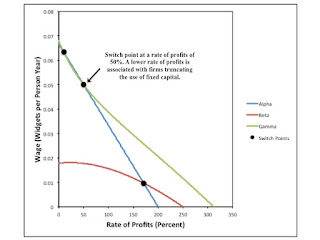
Figure 1: The Choice of Technique in a Model with One Commodity

1.0 Introduction

This post presents a reswitching example in a one-good model. The single produced commodity in the example can be used as both a consumption and a capital good. It is produced by expenditure of labor with its services. It lasts for three production periods, and its technical efficiency varies over the course of its lifetime, when used as a capital good.

I do not remember any comparable numeric example in the literature. If I recall Ian Steedman's 1994 article, he gives instructions for constructing a one-good example, but does not present one. Maybe if I reread it now, I will find it clearer. I have previously worked through a reswitching example, with fixed capital, from J. E. Woods. But that is a multi-commodity model. I have also once echoed Sraffa's analysis of depreciation charges, in a case with constant efficiency.

2.0 Technology

This is an example of fixed capital, a kind of joint production. Three production processes are known by the manager of firms, and they each exhibit constant returns to scale. Each process requires a year to complete, and each process produces new widgets. Table 1 shows the inputs for each process, when operated at a unit level, and Table 2 shows the outputs. For example, process I requires inputs of labor and new widgets. The outputs of process I consist of new widgets and the widgets which provided their services throughout the year it is under operation. Those leftover widgets are one year older, though. Consumers consume new widgets during the year following on their purchase. The physical life of widgets, when providing services for production, is three years. Thus, three processes can be operated in production.

Table 1: Inputs for The Technology

Input	Process
	(I)	(II)	(III)
Labor	10	60	13/2
New Widgets	1/3	0	0
One-Year Old Widgets	0	1/3	0
Two-Year Old Widgets	0	0	1/3

Table 1: Outputs for The Technology

Output	Process
	(I)	(II)	(III)
New Widgets	1	7/12	79/20
One-Year Old Widgets	1/3	0	0
Two-Year Old Widgets	0	1/3	0

Firms are not required to operate all three processes. They can truncate the use of widgets after one or two years. Assume free disposal, that is, that discarding widgets does not incur a cost. Under these assumptions, three techniques are available to produce new widgets, as shown in Table 3.

Table 3: Techniques

Technique	Processes
Alpha	I
Beta	I, II
Gamma	I, II, II

3.0 Price Equations

Managers of widget-producing firms choose the technique, that is, the truncation period, on the basis of cost. As usual, consider a competitive economy, in which workers and firms are free to seek out higher wages and profits, respectively. Revenues and costs are calculated on the basis of a set of prices in which workers and firms have no incentive to move out of one process and into another. Workers receive a common wage of w new widgets per person-year. Assume workers are paid out of the surplus at the end of each year. Firms receive a rate of profits of 100 r percent in operating each process in use. For notational convenience, define R:

R = 1 + r

Let p₁ be the price of a one-year old widget and p₂ the price of a two-year old widget.

I confine the systems of price equations for the Alpha and Beta techniques to an appendix. Accordingly, assume the Gamma technique is in use. The wage, prices, and the rate of profits must satisfy a system of three equations:

(1/3)R + 10 w = 1 + (1/3) p₁

(1/3) p₁ R + 60 w = 7/12 + (1/3) p₂

(1/3) p₂ R + (13/2) w = 79/20

Given the rate of profits below some maximum, one can solve for the wage:

w_γ = (60 R² + 35 R + 237 - 20 R³)/(10 (60 R² + 360 R + 39))

The price of two-year old and one-year old widgets fall out:

p_{2, γ} = (237 - 390 w_γ)/(20 R)

p_{1, γ} = (7 + 4 p_{2, γ} - 720 w_γ)/(4 R)

If you feel like it, you can substitute on the Right Hand Sides of the above two equations so as to express prices as functions exclusively of the rate of profits.

4.0 Choice of Technique

I have explained above how to find the wage, as a function of the rate of profits, when the Gamma technique is in use. The wage-rate of profits curves for the Alpha and Beta technique are, respectively:

w_α = (3 - R)/30

w_β = (12 R + 7 - 4 R²)/(120 (R + 6))

Figure 1 graphs all three wage curves. The cost-minimizing technique, at any given rate of profits, is the technique on the outer envelope of the wage curves. The switch points between the Alpha and Gamma techniques are at rates of profits of 10% and 50%. Below 10% and above 50%, the Gamma technique is cost-minimizing. Widgets are used in production processes to the extent of their physical life. Between these rate of profits, the Alpha technique is cost minimizing. The use of widgets, as capital goods, is truncated after one year. For what it is worth, the switch point between the Alpha and Beta techniques, within the outer envelope, is at a rate of profits of 41/24, approximately 171%.

4.1 A Direct Method with Alpha Prices

In the general theory of joint production, an analysis of the choice of technique cannot generally be based on wage-rate of profits curves. Such an analysis does work in this model of fixed capital. But I checked it with a more direct method of analysis.

Suppose the Alpha technique is in use. The prices of one-year old and two-year old widgets are zero. The wage is as found from the system of price equations associated with the Alpha technique. Would it pay to produce new widgets with one-year old or two-year old widgets? Figure 2 shows calculations to determine if supernormal profits can be earned with the Beta or Gamma technique.

Figure 2: Supernormal Profits at Alpha Prices

Since the Alpha technique is in use, its net present value is zero. Extra profits are assumed to have been competed away.

If the Beta technique is operated, no extra profits or losses are earned in operating process I under the Beta technique. In operating process II, the services of old widgets are free, and no revenues are received for the two-year old widgets disposed of at the end of the year. At low rates of profits and high wages, the revenues received for new widgets produced with process II do not cover labor costs. At high rates of profits, the opposite is the case. These prices, when wages are low, signal to firms that they can earn extra profits by extending the truncation period one year.

The analysis for the Gamma technique is more cumbersome. Firms can not adopt process III without also operating process II. Accordingly, the net present value for the Gamma technique is found by accumulating all costs and revenues for all three processes to the end of the third year. In such a weighted sum, the revenues for process I are multiplied by (1 + r)², and the revenues for process II are multiplied by (1 + r). At a rate of profits below 10% and above 50%, firms will want to adopt the Gamma technique and produce with old widgets to the end of their physical life.

4.2 A Direct Method with Beta Prices

I find of interest some complications that arise in applying this direct method with wages and prices, as calculated for the Beta price system. Figure 3 shows the net present value for the processes comprising each of the three techniques. At all rates of profits, these prices signal that firms should extend the truncation period, from two years, to the three years specified by the Gamma technique. This is so, even for rates of profits between 10% and 50%. If firms start at a two-year truncation period, they will only find that they need to truncate to one year after first extending production to three years. (See A.3 in the Appendix for graphs associated with the Gamma price system.)

Figure 3: Supernormal Profits at Beta Prices

When the Beta technique is operated, a price must be assigned to the price of a one-year old widget. In the theory of joint production, prices can be negative when calculated for rates of profits below the maximum. (This is not so for pure circular capital models without joint production.) Figure 4 graphs the price of one-year old widgets, under the system of prices associated with the Beta technique. This price is negative for rates of profits of approximately 171%. Confine your attention to the Alpha and Beta techniques for a second. The negative price of one-year old widgets signals firms that it is profitable to truncate production from two years to one year.

Figure 4: Price of One-Year Widget with Beta Technique

The application of a direct method for comparing costs and revenues for techniques of production confirms, in the context of this model of fixed capital, the results of constructing the outer envelope curve from the wage-rate of profits curves for the techniques.

5.0 Conclusion

The literature on macroeconomics contains many models with aggregate production functions and in which the one produced commodity can be either consumed by households or used as a capital good in further production. And, in many of these models, this capital good depreciates over many periods. These models are one-good models, in the sense of this post. Some mainstream economists ignorantly assert that the Cambridge Capital Controversy was exclusively about problems in aggregating capital goods. Since mainstream economists are aware of aggregation issues, they somehow conclude they are justified in ignoring the controversy. I usually refute this rot by pointing out consequences for microeconomics of the analysis of the choice of technique. This post takes an alternative approach. It examines a highly aggregated model. And issues related to Sraffa effects arise in the one-good model, too.

This example also has a bearing on a misunderstanding common among the Austrian school of economics. Böhm Bawerk, at least, thought of production processes taking a longer amount of time as being more capital intensive and, therefore, more productive, in some sense. Firms are supposedly restricted in how willing they are to temporally extend production processes because of the scarcity of capital, as reflected in the interest rate. If households were less impatient and more willing to save, the interest rate would fall and firms would adopt longer processes. One can find many Austrian school economists (for example, Hayek in the 1930s) rejecting the idea that there exists a meaningful quantitative measure of roundaboutness or the period of production, whether independent of prices or not. But Austrian school economists generally retain a sense that the theory is insightful and somehow qualitatively true. The numeric example challenges this idea. One would think that a truncation of the production process, with the capital good not reaching its physical lifetime, is unambiguously less roundabout. As noted in Figure 1, for one switch point in the example, such a truncation can be associated with a lower interest rate.

Appendix A

I confine various mathematical details to this appendix.

A.1 Alpha Price Equations

If the Alpha technique is in use, the prices of one-year old and two-year old widgets is zero:

p_{1, α} = p_{2, α} = 0

The wage and the rate of profits are related by the coefficients of production for process I:

(1/3)R + 10 w = 1

The wage, under the Alpha technique, can be expressed as a function of the rate of profits, as illustrated in Figure 1.

A.2 Beta Price Equations

If the Beta technique is in use, the price two-year old widgets is zero:

p_{2, β} = 0

A system of two equations arises for the Beta technique:

(1/3)R + 10 w = 1 + (1/3) p₁

(1/3) p₁ R + 60 w = 7/12

The wage as a function of the rate of profits, for the Beta technique, is also illustrated above. The price of one-year old widgets is:

p_{1, β} = R + 30 w_β - 3

A.3 Direct Method with Gamma Prices

This section presents two graphs with wages and the rate of profits found from the system of prices for the Gamma technique. Figure 5 shows the net present value of truncating the use of widgets after one, two, or three years. For all techniques, revenues and costs are accumulated, at the going rate of profits to the end of the last year in which widgets are produced with the technique. The net present value for operating the Alpha technique (truncating after one year) is positive between the switch points at rates of profits of 10% and 50%.

Figure 5: Supernormal Profits at Gamma Prices

Figure 6 shows the prices of one-year old and two-year old widgets for the solution to the Gamma price system. Although not very easy to see in the graph, the price of one-year old widgets is negative at rates of profits between 10% and 50%.

Figure 6: Price of Widgets with Gamma Technique

References

• Ian Steedman. 1994. 'Perverse' Behaviour in a 'One Commodity' Model. Cambridge Journal of Economics, V. 18, No. 3: pp. 299-311.