On The Emergence of Multiple Cost-Minimizing Techniques

Figure 1: Wage Curves and Rent for an Example of Intensive Rent

The analysis of the choice of technique has above always been based on the construction of a wage-rate of profits frontier. Given a technology in which requirements for use can be satisfied, prices of production for an eligible technique are uniquely determined by the given rate of profits. If the rate of profits is in a range where such prices are non-negative for at least one technique, one of the techniques is uniquely cost-minimizing, except at switch points. This property does not necessarily hold in models of general joint production. The first subsection of the first non-introductory chapter on joint production in Bidard (2004) has the title "Not amused". An examination of local perturbations in an example of intensive rent illustrates surprising possibilities.

Table 1 presents coefficients of production, in which an example from D'Agata (1983) has been extended to include structural economic dynamics. Only one type of land exists, and three processes are known for producing corn on it. The scarcity of land is shown by the possibility of two corn-producing processes being operated side-by-side in the cost-minimizing technique.

Table 1: The Coefficients of Production

Input	Industry
	Iron	Steel	Corn
	I	II	III	IV	V
Labor	1	1	1	(11/5) e1-σ t	e1-φ t
Land	0	0	1	e1-σ t	e1-φ t
Iron	0	0	1/10	(1/10) e1-σ t	(1/10) e1-φ t
Steel	0	0	2/5	(1/10) e1-σ t	(1/10) e1-φ t
Corn	1/10	3/5	1/10	(3/10) e1-σ t	(2/5) e1-φ t

Following D'Agata, assume that one hundred acres of land are available and that net output consists of 90 tons iron, 60 tons steel, and 19 bushels corn. The net output is also the numeraire. All three commodities must be produced for any composition of net output. Table 2 lists the available techniques. Only Alpha, Delta, and Epsilon are feasible for the parameter ranges considered. Not all land is farmed and only one corn-producing process is operated under Alpha. Two corn-producing processes are operated together under Delta and Epsilon.

Table 2: Techniques

Technique	Processes
Alpha	I, II, III
Beta	I, II, IV
Gamma	I, II, V
Delta	I, II, III, IV
Epsilon	I, II, III, V
Zeta	I, II, IV, V

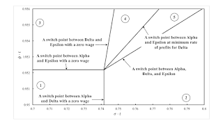
Figure 1 shows the wage curves for feasible techniques at a selected parametrization. I take the wage curve for a technique to be defined only for non-negative rates of profits at which the wage, rent per acre, and the prices of produced commodities are non-negative. The wage is negative for Delta for rates of profits below that at the switch point, and rent is negative for rates of profits greater than that at the switch point. Rent is negative for Epsilon for rates of profits less than at the switch point, and the wage is negative for greater rates of profits. Thus, the switch point is the only point on the wage curves for Delta and Epsilon. The switch point is a fluke in two ways. It is a switch point for three techniques, not two. And it is on the axis for the rate of profits.

Figure 2 shows a partition of the parameter space around this fluke case. An intersection of three wage curves over the axis for the rate of profits is a combination of three pairs of wage curves intersecting over the axis for the rate of profits. These three fluke cases are the partitions between regions 1 and 2, regions 1 and 3, and regions 3 and 4. The partition between regions 2 and 5 is associated with the fluke case of three wage curves intersecting at a non-negative rate of profits. The partition between regions 4 and 5 illustrates a fluke switch point specific to models of rent.

Figure 2: A Part of Parameter Space

Regions 2, 4, and 5 illustrate the possible non-uniqueness and non-existence of a cost-minimizing technique. For concreteness, consider the point in region 4 with the wage curves and variation in rent per acre illustrated in Figure 3. For rates of profits up to the first switch point, Alpha is cost-minimizing. Epsilon is cost-minimizing between the switch points, and Delta is also cost-minimizing for high rates of profits in this range. Beyond the second switch point, no technique is cost-minimizing. Whether or not land is scarce depends on the distribution of income.

Figure 3: Wage Curves and Rent for Region 4

How can one determine which techniques are cost-minimizing for a given rate of profits? Given the technique and the rate of profits, the costs of the capital goods, the rent on land, and wages can be summed for a unit level for each process. Iron, steel, and corn inputs incur the going rate of profits in this sum. The difference between the revenues and this sum is the extra profits obtained in operating a process. By definition, no process comprising the technique yields extra profits. The technique is cost-minimizing if extra profits cannot be obtained by operating any other process.

For the parameters illustrated in Figure 3, extra profits are obtained by operating process IV or V at Alpha prices for a rate of profits greater than that at the first switch point. Alpha is only cost minimizing at a lower rate of profits. Figure 4 depicts the extra profits available from each corn-producing process at Delta and Epsilon prices. The range of rates of profits in which each technique is cost-minimizing is indicated, and these ranges overlap. For some rates of profits greater than the rate of profits at the second switch point, prices of production indicate that Epsilon should be adopted when prices of production for Delta prevail and that Delta should be adopted when prices of production for Epsilon prevail. This circuit is a manifestation of the non-existence of a cost-minimizing technique.

Figure 4: Extra Profits for the Delta and Epsilon Techniques

The cost-minimizing technique is not unique for some rates of profits in regions 2 and 5, as well as in region 4. Even though prices of production are positive for some feasible techniques, no cost-minimizing technique may exist. Table 3 summarizes how cost-minimizing techniques vary with the rate of profits in each of these five numbered regions.

Table 3: Properties of Regions in the Parameter Space

Region	Range	Technique	Notes
1	0 ≤ r ≤ rmax, α	Alpha	No rent is paid.
2	0 ≤ r ≤ rmin, δ	Alpha	No rent is paid.
	rmin, δ ≤ r ≤ r1	Alpha, Delta	The wage curve for Delta slopes up, and rent decreases with the rate of profits.
3	0 ≤ r ≤r1	Alpha	No rent is paid.
	r1 ≤ r ≤ rmax, ε	Epsilon	Rent increases with the rate of profits.
4	0 ≤ r ≤r1	Alpha	No rent is paid.
	r1 ≤ r ≤ rmin, δ	Epsilon	Rent increases with the rate of profits.
	rmin, δ ≤ r ≤ r2	Delta, Epsilon	The wage curve for Delta slopes up. Rent decreases with the rate of profits for Delta and increases for Epsilon.
5	0 ≤ r ≤rmin, δ	Alpha	No rent is paid.
	rmin, δ ≤ r ≤ r1	Alpha, Delta	The wage curve for Delta slopes up, and rent decreases with the rate of profits.
	r1 ≤ r ≤ r2	Delta, Epsilon	The wage curve for Delta slopes up. Rent decreases with the rate of profits for Delta and increases for Epsilon.

Whether or not land obtains a rent can depend on the distribution of income. For a low-enough rate of profits in regions 2, 3, 4, and 5, the first three processes are operated. Iron, steel, and corn are each produced with one process, and land obtains no rent. For a higher rate of profits, the Delta or Epsilon technique can be cost-minimizing. Corn is produced by two processes, and scarce land obtains a rent. Even if the requirements for use can feasibly be satisfied with some land not farmed, the cost-minimizing technique may be such that two processes are operated side-by-side on land, with no land lying fallow.

The reverse substitution of labor, reswitching, capital reversing, the association of the truncation of the economic life of machine with a more capital-intensive technique, a divergence between the order of fertility and the order of rentability, the variation in the existence of rent with the rate of profits or the wage, and the non-uniqueness and the non-existence of a cost-minimizing technique are not fluke cases. These posts demonstrate this conclusion by contrasting these possibilities with genuine fluke cases.

An Extensive Rent Example

Figure 1: Wage Curves and Rent for an Example of Extensive Rent

The analysis of the choice of technique in models of extensive rent can be based on the construction of wage curves, even though the outer envelope does not represent the cost-minimizing technique. The orders of fertility and rentability are emphasized here. The order of fertility is the order in which different qualities of land are introduced into production as requirements for use expand. The order of rentability specifies the sequence of different qualities of lands from high rent per acre to low rent per acre. Both orders may vary with the distribution of income. Table 1 presents coefficients of production for an example. Technical progress is assumed to reduce coefficients of production in each of the corn-producing processes, at different rates.

Table 1: The Coefficients of Production

Input	Iron Industry	Corn Industry
	I	II	III	IV
Labor	1	(5191/5770)e1-φ t	(305/494) e1-θ t	(3/2)e1-σ t
Type 1 Land	0	e1-φ t	0	0
Type 2 Land	0	0	e1-θ t	0
Type 3 Land	0	0	0	e1-σ t
Iron	9/20	(1/40)e1-φ t	(3/1976) e1-θ t	(3/20)e1-σ t
Corn	2	(1/10)e1-φ t	(229/494)e1-θ t	(1/3)e1-σ t

The quantity of produced corn is constrained by the available quantities of each type of land. Suppose endowments include one hundred acres of each type of land, a stationary state prevails, and net output is somewhere between 322 and 444 bushels of corn. Then all three types of land must be farmed with the parameters specified in Figure 1. One type will be only partially farmed. The iron-producing process must be operated in each of the three economically viable techniques sustaining such a stationary state. Table 2 describes which type of lands are fully cultivated and which type of land is left partially farrow in each of the Alpha, Beta, and Gamma techniques.

Table 2:

Technique	Land
	Type 1	Type 2	Type 3
Alpha	Fully farmed	Fully farmed	Partially farmed
Beta	Partially farmed	Fully farmed	Fully farmed
Gamma	Fully farmed	Partially farmed	Fully farmed

For a given technique, the rent on a type of land only partially farmed is zero since it is not scarce. The wage curves in the left pane in Figure 1 are constructed from the price equations provided by the iron-producing process and the corn-producing process for the land that pays no rent in each technique. The choice of technique depends on both income distribution and requirements for use (Quadrio-Curzio 1980). Suppose the rate of profits is taken as given. Then the r-order of efficiency or fertility is the order of the wage curves downwards, until requirements for use are satisfied. Since all three types of land must be somewhat cultivated in the example, the wage frontier is the inner envelope of the wage curves. For the illustrated parameters, Alpha is cost-minimizing, and the order of fertility between the switch points is Type 1, Type 2, and Type 3 lands.

One can calculate the cost of capital goods at the given rate of profits and the cost of labor inputs for corn-producing processes on each of Type 1 and Type 2 lands. Since coefficients of production are specified per bushel corn produced, the revenues from each of these processes, at a unit level, are the same as the process operated on Type 1 land. Rent is the difference between revenues and non-land costs on Type 1 and Type 2 lands. Rent per acre is plotted in the right pane for Figure 1. The order of rentability is the order of lands by rent per acres. The order of rentability is the same as the order of fertility between switch points for the given parameters.

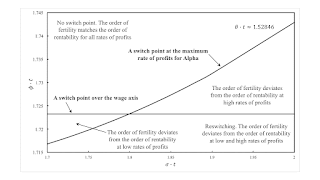
The two fluke switch points in Figure 5 do not lie on the wage frontier. The maximum rate of profits for the wage curve for Alpha is the maximum rate of profits for this example. One of the switch point for the wage curves for the Beta and Gamma techniques is at this maximum rate of profits. As seen in Figure 2, this is another edge case, a fluke that arises in models of extensive rent. By the way, at other parameter ranges the curves for rent as a function of the rate of profits in the right pane in Figure 1 can intersect. The order of rentability can vary with distribution, and fluke cases in which these curves intersect at a maximum rate of profits or a rate of profits of zero can arise.

Figure 2: The Parameter Space

Figure 2 illustrates a region of the parameter space around this fluke case. To the northwest, one switch point between the wage curves for Beta and Gamma has vanished over the wage axis, and the other is at a rate of profits exceeding the maximum rate of profits for Alpha. The order of fertility matches the order of rentability. The southwest is of a reswitching example. For such small perturbations, the order of rentability does not change in this example. Thus, the order of fertility matches the order of rentability only at intermediate rates of profits with reswitching here. The northeast and southwest also illustrate parameters for which the order of fertility varies with the rate of profits. The order of fertility varies from the order of rentability at one or the other extreme, as indicated.

The reverse substitution of labor, reswitching, capital reversing, the association of the truncation of the economic life of machine with a more capital-intensive technique, and a divergence between the order of fertility and the order of rentability are not fluke cases. These posts demonstrate this conclusion by contrasting these possibilities with genuine fluke cases.

Fixed Capital And The Emergence Of Reswitching

Figure 1: A Wage Frontier With A Fluke Switch Point

A fluke example with fixed capital illustrates the emergence of the reswitching of techniques. Table 1 presents coefficients of production in a perturbation of an example from Schefold (1980). With the first process, workers, under the direction of mangers of firms, manufacture new machines. The remaining two processes are used to produce corn. The last process requires an input of an old machine, which is jointly produced with corn by the second process. Corn is both a consumption good and a capital good, insofar as it is an input into all three processes. Technology improves in this example, as usual, with an exponential decline in specified coefficients of production.

Table 1: The Coefficients of Production

Input	Machine Industry	Corn Industry
		One Process	Another Process
Labor	(1/10)e1-σ t	(43/40) e1-φ t	e1-φ t
Corn	(1/16)e1-σ t	(1/16) e1-φ t	(1/4)e1-φ t
New Machines	0	1	0
Old Machines	0	0	1
Output
Corn	0	1	1
New Machines	1	0	0
Old Machines	0	1	0

The choice of technique corresponds here to the choice of the economic life of the machine. This lifetime is truncated to one year for the Alpha technique, while the machine is operated for its full physical life of two years under the Beta technique. In a pure fixed capital model, the choice of technique can be analyzed by the construction of the wage frontier. The cost-minimizing technique at a given rate of profits has a wage curve on the outer frontier, as illustrated by Figure 1 for a specified parametrization. Managers of firms are willing to operate the machine for two years for any feasible rate of profits. At the maximum wage or a rate of profits of zero, the Alpha technique is also cost-minimizing. The single switch point is a fluke in two ways. First, it lies on the wage axis. Second, the wage curves are tangent at the switch point.

The left pane in Figure 2 depicts a part of the parameter space for this example. Although not apparent to the eye, a thin wedge between two partitions extends to the northeast of the point for the parameters corresponding to Figure 1. At the upper edge of this wedge, the two wage curves for the techniques are tangent at a switch point. The example is of reswitching below this partition and within this wedge. Schefold's example lies to the northeast off the graph, when σ t and φ t are both unity. At the lower edge of this wedge, the switch point with the lower rate of profits is on the wage curve. The pane on the right in Figure 2 shows the vertical difference between these two partitions so as to convince the reader of the existence of this region with reswitching.

Figure 2: A Part of a Parameter Space

Reswitching demonstrates the well-known conclusion that no coherent marginal productivity theory of distribution exists. The economic life of the machine is the full two years here for a low and high rate of profits. Truncation occurs for a range of intermediate rates of profits. The specification of which technique is cost-minimizing can be consistent with vastly different functional distributions of income, with other techniques being cost-minimizing for less extreme distributions. Marginal productivity is, at best, an analysis of the choice of technique within a more general framework.

The switch point at the higher rate of profits in the reswitching region of the parameter space illustrates capital-reversing. Around this switch point, a lower rate of profits is associated with the adoption of a less capital-intensive, cost-minimizing technique. At any rate of profits, inputs into production in a stationary state can be evaluated and these evaluations summed for each technique. The ratio of capital per worker, for example, is an index of the capital intensity of a technique. A more capital-intensive technique produces more output per worker, but its adoption is not necessarily encouraged by a lower rate of profits or interest rate. In other words, A higher wage is associated with the adoption of a technique that requires a greater input of labor per bushel corn produced net throughout the economy. Capital-reversing has been shown to occur in other examples without reswitching on the wage frontier. Harcourt (1972) surveys the controversy in which economists, such as Paul Samuelson and Robert Solow, in Cambridge, Massachusetts, struggled to accept these conclusions drawn by other economists, such as Joan Robinson and Piero Sraffa, at the University of Cambridge.

Consider the region to the southeast in the part of the parameter space illustrated in the left pane of Figure 2. A single switch point exists on the wage frontier. Around this switch point, a lower rate of profits is associated with the adoption of a technique with a greater value of capital per person-year and a greater output per worker. Nevertheless, truncating the operation of the machine for one year is associated with a more capital-intensive technique. The invalidity of Austrian capital theory does not even need the phenomena of reswitching and capital-reversing for its demonstration.

No switch points exist in the northwest of the part of the parameter space graphed in Figure 2, and the machine is operated for its full physical life of two years for any feasible distribution of income.

The reverse substitution of labor, reswitching, capital reversing, the association of the truncation of the economic life of machine with a more capital-intensive technique are not fluke cases. These posts demonstrate this conclusion by contrasting these possibilities with genuine fluke cases.

The Emergence Of The Reverse Substitution Of Labor

Figure 1: A Wage Frontier With Two Fluke Switch Points

This post presents an example with circulating capital alone. Table 1 presents the technology for an economy in which two commodities, iron and corn, are produced. One process is known for producing iron, and two are known for producing corn. Each process is specified by coefficients of production, that is, the required inputs per unit output. The Alpha technique consists of the iron-producing process and the first corn-producing process. Similarly, the Beta technique consists of the iron-producing process and the second corn-producing process. At any time, managers of firms face a problem of the choice of technique.

Table 1: The Coefficients of Production

Input	Iron Industry	Corn Industry
		Alpha	Beta
Labor	a0,1 = 1	a0,2α = 0.7174 e-σ t	a0,2β = 1.282 e-φ t
Iron	a1,1 = 9/20	a1,2α = 0.001764 e-σ t	a1,2β = 0.3375 e-φ t
Corn	a2,1 = 2	a2,2α = 0.5386 e-σ t	a2,2β = 0.135 e-φ t

Technical progress, as in structural economic dynamics (Pasinetti 1981), results in decreasing coefficients of production. The coefficients in each corn-producing process decrease at the same rate, but vary between the processes. With wages paid out of the surplus product at the end of the period of production, the wage curves for the two techniques are depicted in Figure 1 for a particular parametrization of the coefficients of production. At this moment in time, the Beta technique is cost-minimizing for any feasible distribution of income. If the wage is zero and the workers live on air, the Alpha technique is also cost-minimizing.

A switch point is defined in this model to be an intersection of the wage curves. These switch points are fluke cases in that almost any variation in the model parameters destroys their interesting properties. A switch point exists at a rate of profits of -100 percent only along a knife edge in the parameter space (Figure 2). Likewise, a switch point exists on the axis for the rate of profits only along another knife edge. The illustrated example, with two fluke switch arises at a single point in the parameter space, where these two partitions intersect.

Figure 2: The Parameters Space for the Reverse Substitution of Labor

Figure 2 depicts a partition of the parameter space around the point with these two fluke switch points. Above the more steeply-sloping locus, the switch point on the axis for the rate of profits has disappeared below the axis. The Beta technique is cost-minimizing for all feasible non-negative rates of profits. Below this locus, the Alpha technique is cost-minimizing for a low enough wage or a high enough feasible rate of profits.

In the north east, the switch point at a negative rate of profits occurs at a rate of profits lower than 100 percent. Around the switch point at a positive rate of profits, a lower wage is associated with a corn-producing process with the larger coefficient for labor. That is, a_0,2^α(σ t) > a_0,2^β(φ t).

In the south east of Figure 2, the switch point for a positive rate of profits exhibits the reverse substitution of labor. Around this switch point, a lower wage is associated with the adoption of a process producing the consumer good in which less labor is employed per unit of gross output. The other switch point exists for a rate of profits between -100 percent and zero. Steedman (2006) presents examples with this phenomenon in models with other structures.

Qualitative changes in the wage frontier exist in the parameter space away from the part graphed in Figure 2. The analysis presented here is only local to the depicted fluke case.

Decades Of Empirical Evidence

I did not always think that mainstream economists are mostly socialized to be unlettered knaves, deficient in mathematics and logic. It took decades of empirical evidence.

These links are mostly to tedious and petty stuff, more for my own archiving. Lots of weird stuff comes from non-economists. Sometimes you will find a poster not necessarily defending me, but trying to get some other poster to say something substantial. Some, like Tim Lambert, do not even seem to care about economics. The misrepresentations by mainstream economists of what they and others say is not confined to discussions with me. Some serious people, like David Graeber, appear in these discussions independent of me.

• Poor teaching of econ (August 2007)
• Failure of neoclassical economics (January, 2006).
• Baumol, Kolakowski, Schumpeter: Bohm Bawerk Mistaken (November 2005).
• Bush tax cut and small businesses (October 2004).
• Edward Prescott, Idiot (October 2004).
• No Mainstream Economist Will Acknowledge Here Math In This Post Is Correct (July 2004).
• Calculation of GDP, Productivity (December 2003).
• Death Rattle Of Neoclassical Theory Of Value (September 2003)
• The economics of free choice (August 2003)
• John Lott (June 2003).
• Reminder: Wages, Employment Not Determined By Supply, Demand (May 2003).
• Some comments on Robert Vienneau's LTV document (April 2003). My FAQ on the LTV.
• Smith And Hegel Agree. Stigler A Hack? (February 2003).
• A Sraffian Interpretation Of Marx (January 2003). My essay.
• Liebowitz Unchained (November 2002).
• Wages, Employment Still Not Determined By Supply And Demand (October 2002).
• Wages, employment not determined by supply, demand (April 2002).
• Debunking Debunking Economics (March 2002).
• Neoclassical Economics Decomposing (March 2002).
• David Landes (February 2002).
• Film criticism at Notre Dame (February 2002).
• Debunking Vienneau (January 2002).
• Paradocs (July 2001).
• Is Boulder Dam capital? (December 2000)
• Response to Scott Moss (March 2000).
• Do Factor Markets Exist? (November 1998).
• LTV FAQ (Part 1 of 6) (November 1998).
• Reswitching and the Cambridge Capital Controversy (October 1998).

I think twitter shows that many with training in economics, science, or mathematics realize that "Mainstream economics is replete with ideas that 'everyone knows' to be true, but that are actually arrant nonsense" (Jeremy Rudd). Maybe I had a small part in this realization.

Update 12 July 2022: Added a link.