Example With Four Normal Forms For Bifurcations Of Switch Points

Figure 1: A Blowup of a Bifurcation Diagram

1.0 Introduction

I have been working on an analysis of structural economic dynamics with a choice of technique. Technical progress can result in a variation in the switch points and the succession of techniques with wage curves on the outer wage frontier. I call such a variation a bifurcation, and I have identified normal forms for four generic bifurcations. This post prevents an example in which all four generic bifurcations appear.

2.0 Technology

The example in is one of an economy in which four commodities can be produced. These commodities are called iron, copper, uranium, and corn. The managers of firms know of one process for producing each of the first three commodities. They know of three processes for producing corn. Table 1 specifies the inputs required for a unit output for each of these six processes. Each column specifies the inputs needed for the process to produce a unit output of the designated industry. Variations in the parameters a_{11, β} and a_{11, γ} can result in different switch points appearing on the frontier.

Table 1: The Technology for Three of Four Industries

Input	Industry
	Iron	Copper	Uranium
Labor	1	17,328/8,281	1
Iron	1/2	0	0
Copper	0	a11, β	0
Uranium	0	0	a11, γ
Corn	0	0	0

Three processes are known for producing corn (Table 2). As usual, these processes exhibit CRS. And each column specifies inputs needed to produce a unit of corn with that process.

Table 2: The Technology the Corn Industry

Input	Process
	Alpha	Beta	Gamma
Labor	1	361/91	3.63505
Iron	3	0	0
Copper	0	1	0
Uranium	0	0	1.95561
Corn	0	0	0

3.0 Technical Progress

3.1 Progress in Copper Production

Consider the variation in the number and location of switch points as the coefficient of production for the input of copper per unit copper produced, a_{11, β}, falls from over 48/91 to around 1/4. In this analysis, the coefficient of production for the input of uranium per unit uranium produced, a_{11, γ}, is set to 3/5. This variation in a_{11, β}, while all other coefficients of production are fixed, describes a type of technical progress in the copper industry.

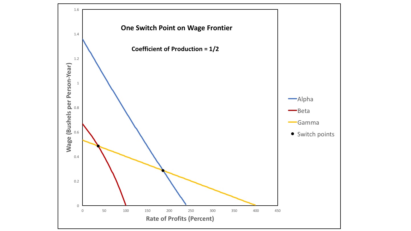
Figure 2 shows the configuration of wage curves near the start of this story. The Gamma technique is never cost-minimizing. For all feasible rates of profits, the wage curve for the Gamma technique falls within the wage frontier. For a parameter value of a_{11, β} of 48/91, the Alpha technique is always cost-minimizing. A single switch point exists, at which the wage curve for the Beta technique is tangent to the wage curve for the Alpha technique, and the Beta technique is also cost-minimizing. I call a configuration of wage curves like that in Figure 2 a reswitching bifurcation. For a slightly lower value of a_{11, β}, two switch points would emerge. The Alpha technique would be cost-minimizing for low and high rates of profits, with the Beta technique cost-minimizing at intermediate rates of profits.

Figure 2: A Reswitching Bifurcation

Figure 3 shows the configuration of wage curves when a_{11, β} has fallen to one half. The interval with high rates of profits where the Alpha technique is uniquely cost-minimizing has vanished. The switch point between Alpha and Beta at high rates of profits occurs at a wage of zero. I call Figure 3 an example of a bifurcation around the axis for the rate of profits. For a slightly smaller value of a_{11, β}, the switch point on the axis would vanish, and only one switch point would exist, in this example, for a non-negative wage.

Figure 3: A Bifurcation around the Axis for the Rate of Profits

Suppose the coefficient of production a_{11, β} were to fall to approximately 0.31008. Figure 4 shows the resulting configuration of wage curves. The Beta technique is cost-minimizing for all feasible positive rates of profit. A single switch point exists, between Alpha and Beta, on the wage axis. If a_{11, β} were to fall even further, no switch points would exist, and Beta would also be cost-minimizing for a rate of profits of zero. I call this an example of a bifurcation around the wage axis.

Figure 4: A Bifurcation around the Wage Axis

Figures 5 and 6 summarize the above discussion. The coefficient of production a_{11, β} is plotted on the abscissa in each figure. The rates of profits and the wage, respectively, are plotted on the ordinate. Switch points are graphed. The maximum rates of profits for the Alpha and Beta technique are plotted in Figure 5. In Figure 6, the maximum wages for Alpha and Beta are plotted. Each of the three bifurcations in Figure 2, 3, and 4 is shown as a thin vertical line in Figures 5 and 6. The wage curve for the Beta techniques moves outward as one passes from the right to the left in the figures. One can see the single switch point becoming two, and the distance between the two, in terms of either the rate of profits of the wage, becoming greater. The rate of profits for one switch point eventually exceeds the maximum rate of profits and disappears. The rate of profits for the other switch point falls below zero, leaving Beta cost-minimizing for all feasible rates of profits and wages. In short, structural economic dynamics, for the case examined here, can be summarized in either one of these two graphs.

Figure 5: A Bifurcation Diagram for Technical Progress in the Copper Industry

Figure 6: A Bifurcation Diagram for Technical Progress in the Copper Industry

3.2 Progress in Uranium Production

An analysis of technical progress in the uranium industry illustrates another type of bifurcation. Let a_{11, β} be set to 51/100, and let the coefficient of production for the input of uranium per unit uranium produced, a_{11, γ}, fall from around 0.55 to 0.4. Figure 7 shows the configuration of wage curves when a_{11, γ} is approximately 0.537986. The wage curves for Alpha and Beta exhibit reswitching. The wage curve for the Gamma technique also intersects the switch point at the lower rate of profits. I call such a configuration of wage curves a three-technique bifurcation. Aside from the switch point, the Gamma technique is never cost-minimizing.

Figure 7: A Three Technique Bifurcation

As a_{11, γ} decreases, the wage curve for the Gamma technique moves outward. At an intermediate value, the wage curve for Gamma intersects the wage curves for Alpha and Beta at different switch points. The reswitching example is transformed into one of capital reversing without reswitching.

Figure 8 displays a case where the wage curve for Gamma has moved outwards until it intersects the other switch point for the reswitching example. Other than at the switch point, the Beta technique is not cost minimizing for any feasible rate of profits. Figure 8 is also a case of a three-technique bifurcation.

Figure 8: Another Three Technique Bifurcation

Figure 9 is a bifurcation diagram illustrating this analysis of technical progress in the uranium industry. It graphs the rate of profits against the coefficient of production a_{11, γ}. Switch points on the wage frontier, as well as the maximum rates of profits for the Alpha and Gamma technique, are graphed. The two thin vertical lines toward the right side of the graph are the two three-technique bifurcations. For a slightly lower value of a_{11, γ} than used in Figure 8, this is a reswitching example between Alpha and Gamma. As a_{11, γ} falls even lower, both switch points disappear over the axis for the rate of profits and the wage, respectively, in a graph of wage curves. That is, this example exhibits another illustration of both a bifurcation around the axis for the rate of profits and a bifurcation around the wage axis.

Figure 9: A Bifurcation Diagram for Technical Progress in the Uranium Industry

3.3 Another Bifurcation Diagram

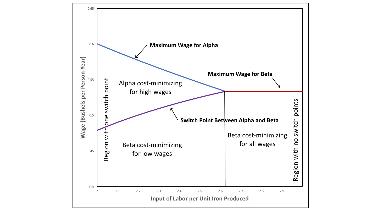
Sections 3.1 and 3.2 each graph switch points against a parameter in the numerical example. A more comprehensive analysis would consider all possible combinations of valid parameter values. One would need to draw a twelve-dimensional space. A part of the space defined by feasible combinations of positive values of a_{11, β} and a_{11, γ} is illustrated in Figure 10, instead Eleven regions are numbered in the figure. Figure 1 enlarges part of Figure 10 and labels the loci dividing regions with specific types of bifurcations.

Figure 10: A Bifurcation Diagram for the Parameter Space

Each numbered region contains an interior. For points in the interior of a region, a sufficiently small perturbation of the coefficients of production a_{11, β} and a_{11, γ} leaves unchanged the number and pattern of switch points. The sequence of cost-minimizing techniques along the wage frontier between switch points is also invariant within regions. Accordingly, Table 3 lists switch points and cost-minimizing techniques for each region. The techniques are specified in order, from a rate of profits of zero to the maximum rate of profits. In several regions, such as region 2, the same technique is listed more than once, since it appears on the wage frontier in two disjoint intervals. Each locus dividing a pair of regions is a bifurcation. The reader can check that the labels for bifurcations in Figure 1 are consistent with Table 3.

Table 3: Techniques on the Wage Frontier

Region	Techniques
1	Alpha throughout
2	Alpha, Beta, Alpha
3	Alpha, Beta
4	Beta throughout
5	Alpha, Gamma, Alpha
6	Alpha, Gamma, Alpha, Beta, Alpha
7	Alpha, Gamma, Beta, Alpha
8	Alpha, Gamma, Beta
9	Alpha, Gamma
10	Gamma
11	Gamma, Beta

To aid in visualization, Figures 11, 12, and 13 graph wage curves and switch points on the wage frontier for each of the eleven regions. Within a region, the number of and characteristics of intersections of wage curves not on the frontier can vary. For example, the graph for region 8 in the lower right of Figure 12 shows an intersection between the wage curves for the Alpha and Gamma techniques at a high rate of profits. That second intersection between these wage curves can disappear over the axis for the rate of profits while leaving the sequence, if not the location, of cost-minimizing techniques and switch points on the frontier unchanged.

Figure 11: Wage Curves for Regions 1 through 4

Figure 12: Wage Curves for Regions 5 through 8

Figure 13: Wage Curves for Regions 9 through 11

The numerical example is an instance of the Samuelson-Garegnani model. Variations in the two coefficients of production for the copper industry have no effect on the location of intersections between wage curves for Alpha and Gamma. Thus, one obtains the horizontal lines in Figures 1 and 10. Likewise, variations in a_{11, γ} do not affect intersections between the wages curves for Alpha and Beta. This property results in the vertical lines in the bifurcation diagram. Bifurcations in which wage curves for both Beta and Gamma are involved result in the more or less diagonal curves in Figures 1 and 10.

Section 3.1 tells a tale of technical progress in the copper industry. This story is illustrated by the bifurcation diagrams in Figures 1 and 10. The chosen values for a_{11, β} divide regions 1, 2, 3, and 4. Figure 2 lies along the vertical line dividing regions 1 and 2. Figure 3 illustrates the division between regions 2 and 3, and Figure 4 illustrates the corresponding division between regions 3 and 4. The vertical line towards the left side of Figure 10 is a bifurcation across the wage axis.

Similarly, Section 3.2 illustrates bifurcations along a movement downward in Figures 1 and 10. Such a downward movement would pass through regions 2, 7, 5, 9, and 10. Figure 7 illustrates parameters on the locus dividing regions 2 and 7. Figure 8 illustrates the division between regions 7 and 5. The line dividing regions 5 and 9 is a bifurcation around the axis for the rate of profits, and the line dividing regions 9 and 10 is a bifurcation around the wage axis. All four bifurcations are illustrated in Figure 9.

The above partitioning of the parameter space formed by coefficients of production suggests the existence of bifurcations not yet illustrated. For example, a three-technique bifurcation is located anywhere along the locus dividing regions 6 and 7. This bifurcation differs from the three-technique bifurcations illustrated by Figures 7 and 8. Or consider the point that separates regions 1, 2, 5, and 6. The Alpha technique is cost minimizing for all feasible rates of profits for these coefficients of production. Two switch points exist, and at each one of these switch points another technique is tied with the Alpha technique. The wage curve for the Gamma technique is tangent to the wage curve for the Alpha technique at the switch point with the lower rate of profits. The wage curve for the Beta technique is tangent to the wage curve for the alpha technique at the other switch point. The point on the intersection between the loci dividing regions 2, 6, and 7 is interesting. The coefficients of production specified by this point characterize a three-technique bifurcation in which the wage curves for the Alpha and Gamma techniques are tangent at the appropriate switch point. This discussion has not exhausted the possibilities.

The Concept Of Totality

This post is inspired by current events

"It is not the primacy of economic motives in historical explanation that constitutes the decisive difference between Marxism and bourgeois thought, but the point of view of totality. The category of totality, the all-pervasive supremacy of the whole over the parts is the essence of the method which Marx took over from Hegel and brilliantly transformed into the foundations of a wholly new science. The capitalist separation of the producer from the total process of production, the division of the process of labour into parts at the cost of the individual humanity of the worker, the atomisation of society into individuals who simply go on producing without rhyme or reason, must all have a profound influence on the thought, the science and the philosophy of capitalism. Proletarian science is revolutionary not just by virtue of its revolutionary ideas which it opposes to bourgeois society, but above all because of its method. The primacy of the category of totality is the bearer of the principle of revolution in science.

The revolutionary nature of Hegelian dialectics had often been recognised as such before Marx, notwithstanding Hegel's own conservative applications of the method. But no one had converted this knowledge into a science of revolution. It was Marx who transformed the Hegelian method into what Herzen described as the 'algebra of revolution'. It was not enough, however, to give it a materialist twist. The revolutionary principle inherent in Hegel's dialectic was able to come to the surface less because of that than because of the validity of the method itself, viz. the concept of totality, the subordination of every part to the whole unity of history and thought. In Marx the dialectical method aims at understanding society as a whole. Bourgeois thought concerns itself with objects the arise either from the process of studying phenomena in isolation, or from the division of labour and specialisation in the different disciplines. It holds abstractions to 'real' if it is naively realistic, and 'autonomous' if it is critical."

-- Georg Lukács, History and Class Consciousness (trans. by Rodney Livingstone), MIT Press (1971): pp. 27-28.

A Reswitching Bifurcation, Reflected

Figure 1: Two Bifurcation Diagrams Horizontally Reflecting

1.0 Introduction

This post continues my investigation of structural economic dynamics. I am interested in how technological progress can change the analysis of the choice of technique. I have four normal forms for how switch points can appear on or disappear from the wage frontier, as a result of changes in coefficients of production. This post concentrates on what I call a reswitching bifurcation.

Each bifurcation can be described by how wages curves look around the bifurcation before, at, and after the bifurcation. I claim that, in some sense, order does not matter. For each normal form, bifurcations can exist in either order. I have proven this, for three of the bifurcations, by constructing the normal forms in both orders. This post completes the proof by exhibiting both orders for the reswitching bifurcation.

2.0 Technology

Consider the technology illustrated in Table 1. The managers of firms know of four processes of production. And these processes exhibit Constant Returns to Scale. The column for the iron industry specifies the inputs needed to produce a ton of iron. The column for the copper industry likewise specifies the inputs needed to produce a ton of copper. Two processes are known for producing corn, and their coefficients of production are specified in the last two columns in the table. Each process is assumed to require a year to complete and uses up all of its commodity inputs. Technology is defined in terms of two parameters, u and v. u denotes the quantity of labor needed to produce a unit iron in the iron industry. v is the quantity of labor needed to produce a unit copper.

Table 1: The Technology for a Three-Commodity Example

Input	Industry
	Iron	Copper	Corn
			Alpha	Beta
Labor	u	v	1	361/91
Iron	1/2	0	3	0
Copper	0	48/91	0	1
Corn	0	0	0	0

As usual, this technology presents a problem of the choice of technique. The Alpha technique consists of the iron-producing process and the corn-producing process labeled Alpha. Similarly, the Beta technique consists of the copper-producing process and the corn-producing process labeled Beta.

3.0 Selected Configurations of Wage Curves

3.1 A Reswitching Bifurcation

Consider certain specified parameter values for the coefficients of production denoting the amount of labor needed to produce one unit of iron and one unit of copper. In particular, let u be 1, and let v be 17,328/8,281. Figure 2 graphs the wage curves for the two techniques in this case.

Figure 2: Wage Curves at the Bifurcation

I call this case a reswitching bifurcation. Like all bifurcations, it is a fluke case.

3.2 Improvements in Iron Production Around The Reswitching Bifurcation

Consider variations in u, from some parameter larger than its value in the above reswitching bifurcation to some lower value. In this part of the story, the value of v is assumed to be fixed at its value for the bifurcation. The right half of Figure 1, at the top of this post, illustrates this story.

For a high value of u, to the right of the right of Figure 1, the wage curve for Alpha is moved inside its location in Figure 2. The wage curves for the Alpha and Beta techniques intersect at two points. It is a reswitching example. A fall in u is illustrated by a movement to the left on the right side of Figure 1. The two switch points become closer and closer along the wage frontier. The reswitching bifurcation is illustrated by the thin vertical line in Figure 1. For any smaller value of u, the Alpha technique is cost minimizing for all feasible rates of profits or wages.

3.3 Improvements in Copper Production Around The Reswitching Bifurcation

Now consider variations in v, with u fixed at the value for the bifurcation illustrated in Figure 2. Technical progress in the copper industry is illustrated by a movement to the left on the left side of Figure 1. For a high value of v, the wage curve for the Beta technique is inside the wage curve for the Alpha technique. The Alpha technique is cost-minimizing for all feasible rates of profits. As v decreases, the wage curve for the Beta technique moves outward, until it reaches the reswitching bifurcation. For smaller values of v, the example becomes, once again, a reswitching example. A second bifurcation is illustrated on the left side of Figure 1, when the switch point at the higher rate of profits moves across the axis for the wage. The labor input for copper has become so small that the Beta technique is cost-minimizing for any sufficiently large enough wage and small rate of profits.

4.0 Conclusion

The bifurcation depends on a certain relative configuration of wage curves, in which one is tangent to the other at a switch point. Whether technical progress around the bifurcation results in reswitching appearing or disappearing depends on which wage curve is moving outwards faster around the switch point(s). Either order is possible.

Elsewhere

• Nick Hanauer argues for some policies that postulate:
• Income distribution is not a matter of supply and demand or any other sort of economic natural laws.
• That a more egalitarian distribution of income leads to an increased demand and generalized shared prosperity.
• Tom Palley contrasts neoliberalism with an economic theory with an approach with another "theory of income distribution and its theory of aggregate employment determination".
• Elizabeth Bruenig contrasts liberalism with the the left.
• Paul Blest laughs at whining neoliberals
• Chris Lehmann considers how the turn of the US's Democratic Party to neoliberalism lowers its electoral prospects.

Is the distinction between democratic socialism and social democracy of no practical importance at the moment in any nation's politics? I think of the difference in two ways. First, in the United States in the 1970s, leftists had an argument. Self-defined social democrats became Neoconservatives, while democratic socialists found the Democratic Socialists of America (DSA). Second, both are reformists approaches to capitalism, advocating tweaks to, as Karl Popper argued for, prevent unnecessary pain. But social democrats have no ultimate goal of replacing capitalism, while democratic socialists want to end up with a transformed system.

A Fluke Of A Fluke Switch Point

Figure 1: Wage Curves

1.0 Introduction

This post presents an example of the analysis of the choice of technique in competitive markets. The example is one with three techniques and two switch points. The wage curves for the Alpha and Beta techniques are tangent at one of the switch points. This is a fluke. And the wage curves for all three techniques all pass through that same switch point. This, too, is a fluke.

I suppose that the example is one of reswitching and capital-reversing is the least interesting property of the example. Paul Samuelson was simply wrong in labeling such phenomena as perverse. A non-generic bifurcation, like the illustrated one, falls out of a comprehensive analysis of possible configurations of wage curves.

2.0 Technology

The technology in the example has a particularly simple structure. Firms can produce one of three capital goods, which I am arbitrarily labeling iron, copper, and uranium. Table 1 shows the production processes known for producing each metal. One process is known for producing each, and each metal is produced out of inputs of labor and that metal. Each process requires a year to complete, uses up all its material inputs, and exhibits Constant Returns to Scale.

Table 1: The Technology for Three of Four Industries

Input	Industry
	Iron	Copper	Uranium
Labor	1	17,328/8,281	1
Iron	1/2	0	0
Copper	0	48/91	0
Uranium	0	0	0.53939
Corn	0	0	0

Three processes are known for producing corn (Table 2), which is the consumption good. This economy can be sustained by adopting one of three techniques. The Alpha technique consists of the iron-producing process and the corn-producing process labeled Alpha. Similarly, the Beta technique consists of the copper-producing process and the corn-producing process labeled Beta. Finally, the Gamma technique consists of the remaining two processes.

Table 2: The Technology the Corn Industry

Input	Process
	Alpha	Beta	Gamma
Labor	1	361/91	3.63505
Iron	3	0	0
Copper	0	1	0
Uranium	0	0	1.95561
Corn	0	0	0

3.0 The Choice of Technique

The choice of technique is analyzed based on prices of production and cost-minimization. Labor is assumed to be advanced, and wages are paid out of the surplus product at the end of the year. Corn is taken as the numeraire. Figure 1 graphs the wage-rate of profits for the three techniques. The cost-minimizing technique, at a given rate of profits, maximizes the wage. That is, the cost-minimizing techniques form the outer envelope, also known as, the wage frontier, from the wage curves. Aside from switch points, the Alpha technique is cost-minimizing at low and high rates of profits, with the Gamma technique cost-minimizing between the switch points. At switch points, any linear combination of the techniques with wage curves going through that switch point are cost-minimizing.

The wage curve for the Beta technique is a straight line. This affine property results from the Organic Composition of Capital being the same in copper production and in corn production, when the Beta technique is adopted. To help visualization, I also graph the difference between the wage curves (Figure 2). The Beta technique is only cost-minimizing at the switch point at the higher rate of profits. The tangency of the wage curves for the Alpha and Beta techniques is manifested in Figure 2 by the non-negativity of the difference in these curves.

Figure 2: Distance Between Wage Curves

4. Conclusion

I'm sort of proud of this example. I suppose I could, at least, submit it for publication somewhere. But it is only a side effect of a larger project I guess I am pursuing.

I want to introduce a distinction among fluke switch points. Every bifurcation (that is, a change in the sequence of switch points and cost-minimizing techniques along the wage frontier) is a fluke. Some perturbation of a coefficient of production from a bifurcation value will change that sequence. Suppose a perturbation of a coefficient of production not involved in a bifurcation, in some sense, leaves the qualitative story unchanged. One can use the same bifurcation to tell a story about, say, technological progress. This is a generic bifurcation.

Accept, for the sake of argument, that prices of production tell us something about actual prices. The economy is never in an equilibrium, but owners of firms are always interested in increasing their profits. One can never expect observed technology to meet the fluke conditions of a generic bifurcation. But it can tell us something about how the dynamics of income distribution, for example, vary with technological progress.

Suppose one perturbs, in the example, the coefficient of production for the amount of iron needed to produce iron. (I denote this coefficient, in a fairly standard notation, as a_1,1^β.) Then, either the wage curves for the. Alpha and Beta techniques will not intersect at all or they will intersect twice. In the latter case, one can vary a_1,1^γ to find an example in which all three wage curves intersect at one or another of the switch points. But the tangency will be lost. So I consider the fluke point illustrated to be a non-generic bifurcation.

Non-generic bifurcations arise in a complete bifurcation analysis. The model illustrated remains open. Income distribution is not specified. Nevertheless, I think this theoretical analysis can say something to those who are attempting to empirically apply the Leontief-Sraffa model.

Some Unresolved Issues In Multiple Interest Rate Analysis

1.0 Introduction

Come October, as I understand it, the Review of Political Economy will publish, in hardcopy, my article The Choice of Technique with Multiple and Complex Interest Rates. I discuss in this post questions I do not understand.

2.0 Non-Standard Investments and Fixed Capital

Consider a point-input, flow-output model. In the first year, unassisted labor produces a long-lived machine. In successive years, labor and a machine of a specific history are used to produce outputs of a consumption good and a one-year older machine. The efficiency of the machine may vary over the course of its physical lifetime. When the machine should be junked is a choice variable in some economic models.

I am aware that in this, or closely related models, the price of a machine of a specific date can be negative. The total value of outputs at such a year in which the price of the machine of the machine is negative, however, is the difference between the sum of the price of the machine & the consumption good and the price of any inputs, like labor, that are hired in that year. Can one create a numerical example of such a case in which the net value, in a given year, is negative, where that negative value is preceded and followed by years with a positive net value?

If so, this would an example of a non-standard investment. A standard investment is one in which all negative cash flows precede all positive cash flows. In a non-standard investment at least one positive cash flow precedes a negative cash flow, and vice-versa. Non-standard investments create the possibility that all roots of the polynomial used to define the Internal Rate of Return (IRR) are complex. Can one create an example with fixed capital or, more generally, joint production in which this possibility arises?

Does corporate finance theory reach the same conclusions about the economic life of a machine as Sraffian analysis in such a case? Can one express Net Present Value (NPV) as a function combining the difference between the interest rate and each IRR in this case, even though all IRRs are complex? (I call such a function an Osborne expression for the NPV.)

3.0 Generalizing the Composite Interest Rate to the Production of Commodities by Means of Commodities

In my article, I follow Michael Osborne in deriving what he calls a composite interest rate, that combines all roots of the polynomial defining the IRR. I disagree with him, in that I do not think this composite interest rate is useful in analyzing the choice of technique. But we both obtain, in a flow-input, point output model, an equation I find interesting.

This equation states that the difference between the labor commanded by a commodity and the labor embodied in that commodity is the product of the first input of labor per unit output and the composite interest rate. Can you give an intuitive, theoretical explanation of this result? (I am aware that Osborne and Davidson give an explanation, that I can sort of understand when concentrating, in terms of the Austrian average period of production.)

A model of the production of commodities by means of commodities can be approximated by a model of a finite sequence of labor inputs. The model becomes exact as the number of dated labor inputs increases without bound. In the limit, the labor command by each commodity is a finite value. So is the labor embodied. And the quantity for the first labor input decrease to zero. Thus, the composite interest rate increases without bound. How, then, can the concept of the composite interest rate be extended to a model of the production of commodities by means of commodities?

4.0 Further Comments on Multiple Interest Rates with the Production of Commodities by Means of Commodities

In models of the production of commodities by means of commodities, various polynomials arise in which one root is the rate of profits. I have considered, for example, the characteristic equation for a certain matrix related to real wages, labor inputs, and the Leontief input-output matrix associated with a technique of production. Are all roots of such polynomials useful for some analysis? How so?

Luigi Pasinetti, in the context of a theory of Structural Economic Dynamics, has described what he calls the natural system. In the price system associated with the natural system, multiple interest rates arise, one for each produced commodity. Can these multiple interest rates be connected to Osborne's natural multiple interest rates?

5.0 Conclusion

I would not mind reading attempts to answer the above questions.

Switch Points and Normal Forms for Bifurcations

I have put up a working paper, with the post title, on my Social Sciences Research Network (SSRN) site.

Abstract: The choice of technique can be analyzed, in a circulating capital model of prices of production, by constructing the wage frontier. Switch points arise when more than one technique is cost-minimizing for a specified rate of profits. This article defines four normal forms for structural bifurcations, in which the number and sequence of switch points varies with a variation in one model parameter, such as a coefficient of production. The 'perversity' of switch points that appear on and disappear from the wage frontier is analyzed. The conjecture is made that no other normal forms exist of codimension one.

Switch Points Disappearing Or Appearing Over The Axis For The Rate Of Profits

Figure 1: Two Bifurcation Diagrams Horizontally Reflecting

1.0 Introduction

This post continues my investigation of structural economic dynamics. I am interested in how technological progress can change the analysis of the choice of technique. In this case, I explore how a decrease in a coefficient of production can cause a switch point to appear or disappear over the axis for the rate of profits.

2.0 Technology

Consider the technology illustrated in Table 1. The managers of firms know of four processes of production. And these processes exhibit Constant Returns to Scale. The column for the iron industry specifies the inputs needed to produce a ton of iron. The column for the copper industry likewise specifies the inputs needed to produce a ton of copper. Two processes are known for producing corn, and their coefficients of production are specified in the last two columns in the table. Each process is assumed to require a year to complete and uses up all of its commodity inputs. Technology is defined in terms of two parameters, u and v. u denotes the quantity of iron needed to produce a unit iron in the iron industry. v is the quantity of copper needed to produce a unit copper.

Table 1: The Technology for a Three-Commodity Example

Input	Industry
	Iron	Copper	Corn
			Alpha	Beta
Labor	1	2/3	1	2/3
Iron	u	0	1/3	0
Copper	0	v	0	1/3
Corn	0	0	0	0

As usual, this technology presents a problem of the choice of technique. The Alpha technique consists of the iron-producing process and the corn-producing process labeled Alpha. Similarly, the Beta technique consists of the copper-producing process and the corn-producing process labeled Beta.

I make all my standard assumptions. The choice of technique is based on cost-minimization. Consider prices of production, which are stationary prices that allow the economy to be reproduced. A wage curve, showing a tradeoff between wages and the rate of profits, is associated with each technique. In drawing such a curve, I assume that a bushel corn is the numeraire and that labor is advanced. Hence, wages are paid out of the surplus product at the end of the year. The chosen technique, for, say, a given wage, maximizes the rate of profits. The wage curve for the cost-minizing technique at the given wage lies on the outer frontier formed from all wage curves.

3.0 Innovations

I have two stories of technical innovation. In one, improvements are made in the process for producing copper. As a consequence, the wage curve for the Beta technique moves outward. In the other story, improvements are made in the iron industry, and the wage curve for the Alpha technique moves outwards. The bifurcations that occur in the two stories are mirror reflections of one another, in some sense.

3.1 Improvements in Copper Production

Let u be fixed at 1/3 tons per ton. The wage curve for the Alpha technique is a downward sloping straight line. Let v decrease from 1/2 to 3/10. When v is 1/3, the wage curve for the Beta technique is also a straight line. I created the example to have linear (actually, affine) wage curves at the bifurcation for convenience. The bifurcation does not require such.

Figure 2 shows the wage curves when the copper coefficient for copper production is a high value, in the range under consideration. A single switch point exists, and the Alpha technique is cost-minimizing if the rate of profits is high. As v decreases, the switch point moves to a higher and higher rate of profits. (These statements are about the shapes of mathematical functions. They are not about historical processes set in time.) Figure 3 shows the wage curves when v is 1/3. The switch point is now on the axis for the rate of profits. For any non-negative rate of profits below the maximum, the Beta technique is cost-minimizing. Finally, Figure 4 shows the wage curves for an even lower copper coefficient in copper production. Now, there is no switch point, and the Beta technique is always cost-minimizing, for all possible prices of production.

Figure 2: Wage Curves Without Improvement in Copper Production

Figure 3: Wage Curves For A Bifurcation

Figure 4: Wage Curves After Improvements in Copper Production

3.2 Improvements in Iron Production

Now let v be set at 1/3. Let u decrease from 1/2 to 3/10. Figure 5 shows the wage curves at the high end for the iron coefficient in iron production. No switch point exists, and the Beta technique is always cost-minimizing. I thought about repeating Figure 3, for v decreased to 1/3. The same configuration of wage curves, with a bifurcation, appears in this story. Figure 6, shows that the switch point appears for an even lower value of the iron coefficient.

Figure 5: Wage Curves Without Improvement in Iron Production

Figure 6: Wage Curves After Improvements in Iron Production

3.3 Improvements in Both Iron and Copper Industries

I might as well graph (Figure 7) the copper coefficient in copper production against the iron coefficient in iron production. The bifurcation occurs when the maximum rates of profits are identical in the Alpha and Beta technique. In a model with the simple structure of the example, this occurs when u = v. Representative illustrations of wage curves are shown in the regions in the parameter space. A switch point below the maximum rate of profits exists only above the line in parameter space representing the bifurcation.

Figure 7: Bifurcation Diagram for Two Coefficients of Production

The story in Section 3.1 corresponds to moving downwards on a vertical line in Figure 7. The left-hand side of Figure 1, at the top of this post, is another way of illustrating this story. On the other hand, Section 3.2 tells a story of moving leftwards on a horizontal line in Figure 7. The right-hand side of Figure 1 illustrates this story.

Focus on the intersections, in the two sides of Figure 1 of the blue, red, and purple loci. Can you see that, in some sense, they are reflections, up to a topological equivalence?

4.0 Discussion

I have a reswitching example with a switch point disappearing over the axis for the rate of profits. In that example, the disappearing switch point is 'perverse', that is, it has a positive real Wicksell effect. In the examples in Section 3 above, the disappearing or appearing switch point is 'normal', with a negative real Wicksell effect.

Bifurcations Along Wage Frontier, Reflected

Figure 1: Bifurcation Diagram

1.0 Introduction

This post continues a series investigating structural economic dynamics. I think most of those who understand prices of production - say, after working through Kurz and Salvadori (1995) - understand that technical innovation can change the appearance of the wage frontier. (The wage frontier is also called the wage-rate of profits frontier and the factor-price frontier.) Changes in coefficients of production can create or destroy a reswitching example. But, as far as I know, nobody has systematically explored how this happens in theory.

I claim that when switch points appear on or disappear off of the wage frontier, these bifurcations follow a few normal forms. I have been describing each normal form as a story of a coefficient of production being reduced by technical innovation. I further claim that, in some sense, the order of changes along the wage frontier is not specified. One can find an example with a decreasing coefficient of production in which the order is the opposite of some other example of technical innovation with the same normal form.

This post is one of a series providing the proof that order does not matter. The example in this post relates to this previous example.

2.0 Technology

The example in this post is one of an economy in which four commodities can be produced. These commodities are called iron, steel, copper, and corn. The managers of firms know (Table 1) of one process for producing each of the first three commodities. These processes exhibit Constant Returns to Scale. Each column specifies the inputs required to produce a unit output for the corresponding industry. Variations in the parameter v can result in different switch points appearing on the frontier. Each process requires a year to complete and uses up all of its inputs in that year. There is no fixed capital.

Table 1: The Technology for Three of Four Industries

Input	Industry
	Iron	Steel	Copper
Labor	1/2	1	3/2
Iron	53/180	0	0
Steel	0	v	0
Copper	0	0	1/5
Corn	0	0	0

Three processes are known for producing corn (Table 2). As usual, these processes exhibit CRS. And each column specifies inputs needed to produce a unit of corn with that process.

Table 2: The Technology the Corn Industry

Input	Process
	Alpha	Beta	Gamma
Labor	1/2	1	3/2
Iron	1/3	0	0
Steel	0	1/4	0
Copper	0	0	1/5
Corn	0	0	0

Four techniques are available for producing a net output of a unit of corn. The Alpha technique consists of the iron-producing process and the Alpha corn-producing process. The Beta technique consists of the steel-producing process and the Beta process. The Gamma technique consists of the remaining two processes.

As usual, the choice of technique is based on cost-minimization. Consider prices of production, which are stationary prices that allow the economy to be reproduced. A wage curve, showing a tradeoff between wages and the rate of profits, is associated with each technique. In drawing such a curve, I assume that a bushel corn is the numeraire and that labor is advanced. Wages are paid out of the surplus product at the end of the year. The chosen technique, for, say, a given wage, maximizes the rate of profits. The wage curve for the cost-minizing technique at the given wage lies on the outer frontier formed from all wage curves.

3.0 Technical Progress

Figures 2 through 5 illustrate wage curves for different levels of the coefficient of production denoted v in the table. Figure 2 shows that for a relatively high parameter value, the switch point between the Alpha and Gamma techniques is the only switch point on the outer frontier. For continuously lower parameter values of v, the wage curve moves outward. Figure 3 illustration the bifurcation value, a fluke case in which the wage curves for all three techniques intersect in a single switch point. Other than at the switch point, the wage curve for the Beta technique is not on the frontier. But, for a slightly lower parameter value (Figure 4), the wage curve for the Beta technique, along with switch points between the Alpha and the Beta techniques and between the Beta and Gamma techniques, is on the frontier. The intersection between the wage curves for the Alpha and Gamma techniques is no longer on the frontier. Figure 5 illustrates another bifurcation in the example. The focus of this post is not on this bifurcation, in which a switch point disappears over the axis for the rate of profits.

Figure 2: Wage Curves with High Steel Inputs in Steel Production

Figure 3: Wage Curves with Medium Steel Inputs in Steel Production

Figure 4: Wage Curves with Low Steel Inputs in Steel Production

Figure 5: Wage Curves with Lowest Steel Inputs in Steel Production

4.0 Discussion

The bifurcation on the right in Figure 1, at the top of this post, is topologically equivalent to the horizontal reflection of the bifurcation on the right in the equivalent figure in this previous post. (On the other hand, the bifurcations on the upper left in both diagrams are the same normal form, in the same order.)

The bifurcation described in this post is a local bifurcation. To characterize this bifurcation, one need only look at small range of rates of profits and coefficients of production around a critical value. Accordingly, then wage curves involved in the bifurcations could intercept any number of times, in some other example of this normal form, at positive rates of profits. Each of the three switch points involved in the bifurcation could have any direction for real Wicksell effects, positive or negative.

The bifurcation, as depicted in this post, replaces one switch point on the wage curve with two switch points. It could be that the switch point disappearing exhibits capital-reversing, and both of the two new switch points appearing also exhibit capital-reversing. But any of five other other combinations are possible.

The Choice Of Technique With Multiple And Complex Interest Rates

My article with the post title is now available on the website for the Review of Political Economy. It will be, I gather, in the October 2017 hardcopy issue. The abstract follows.

Abstract: This article clarifies the relations between internal rates of return (IRR), net present value (NPV), and the analysis of the choice of technique in models of production analyzed during the Cambridge capital controversy. Multiple and possibly complex roots of polynomial equations defining the IRR are considered. An algorithm, using these multiple roots to calculate the NPV, justifies the traditional analysis of reswitching.

A Switch Point Disappearing Over The Wage Axis

Figure 1: Bifurcation Diagram

1.0 Introduction

In a series of posts, I have been exploring structural economic dynamics. Innovation reduces coefficients of production. Such reductions can vary the number and sequence of switch points on the wage frontier. I call such a variation a bifurcation. And I think such bifurcations, at least if only one coefficient decreases, fall into a small number of normal forms.

One possibility is that a decrease in a coefficient of production results in a switch point appearing over the wage axis, as illustrated here. This post modifies that example such that the switch point disappears over the wage axis with a decrease in a coefficient of production.

2.0 Technology

Accordingly, consider the technology illustrated in Table 1. The managers of firms know of four processes of production. And these processes exhibit Constant Returns to Scale. The column for the iron industry specifies the inputs needed to produce a ton of iron. The column for the copper industry likewise specifies the inputs needed to produce a ton of copper. In this post, I consider how variations in the parameter u affect the number of switch points. Two processes are known for producing corn, and their coefficients of production are specified in the last two columns in the table. Each process is assumed to require a year to complete and uses up all of its commodity inputs.

Table 1: The Technology for a Three-Commodity Example

Input	Industry
	Iron	Copper	Corn
			Alpha	Beta
Labor	21/8	u	1	3/2
Iron	1/4	0	1/4	0
Copper	0	1/5	0	1/5
Corn	0	0	0	0

This technology presents a problem of the choice of technique. The Alpha technique consists of the iron-producing process and the corn-producing process labeled Alpha. Similarly, the Beta technique consists of the copper-producing process and the corn-producing process labeled Beta.

The choice of technique is based on cost-minimization. Consider prices of production, which are stationary prices that allow the economy to be reproduced. A wage curve, showing a tradeoff between wages and the rate of profits, is associated with each technique. In drawing such a curve, I assume that a bushel corn is the numeraire and that labor is advanced. Hence, wages are paid out of the surplus product at the end of the year. The chosen technique, for, say, a given wage, maximizes the rate of profits. The wage curve for the cost-minizing technique at the given wage lies on the outer frontier formed from all wage curves.

3.0 Results

Consider variations in u, the input of labor in the copper industry, per unit copper produced. Figure 1 shows the effects of such variations. For a high value of this coefficient, a single switch point exists. The Alpha technique is cost-minimizing at high wages (or low rates of profits). The Beta technique is cost-minimizing at low wages (or high rates of profits).

Suppose that technical innovations reduce u to 3/2. Then the switch point occurs at the maximum wage. For all positive rates of profits (not exceeding the maximum), the Beta technique is cost-minimizing. At a rate of profits of zero, both techniques (or any linear combination of them) are eligible for adoption by cost-minimizing firms.

A third regime arises when technical innovations reduce u even more. The a technique is cost-minimizing for all feasible rates of profits, including a rate of profits of zero.

4.0 Discussion

So this example has illustrated that the bifurcation diagram at the top of this previous post can be reflected across a vertical line where the bifurcation occurs. An abstract description of a bifurcation in which a switch point crosses the wage axis does not have a direction, in some sense. Either direction is possible.

The illustrated bifurcation is, in some sense, local. The illustrated phenomenon might occur in what is originally a reswitching example. That is, the bifurcation concerns only what happens around a small rate of profit (or near the maximum wage). It is compatible with wage curves that have a second intersection on the frontier at a higher rate of profits. In such a case, the switch point at the higher rate of profits will remain. But the bifurcation will transform it from a 'perverse' switch point to a 'normal' one.

As I understand it, such a bifurcation of a reswitching will be manifested in the labor market with 'paradoxical' behavior. Suppose the first switch point disappears over the wage axis. Around the second switch point, a comparison of long period (stationary) positions will find a higher wage associated with the adoption of a technique that requires less labor per (net) unit output, for the economy as a whole. But, in the corn industry, a higher wage will be associated with the adoption of a technique that requires more labor per (gross) unit corn produced.

This is just one of those possibilities that demonstrates the Cambridge Capital Controversy is not merely a critique of aggregation, macroeconomics, and the aggregate production function. It has implications for microeconomics, too.

Piers Anthony, Neoliberal

A Spell for Chameleon, the first book of the Xanth series, shows that Piers Anthony is a neoliberal¹. Magicians are important characters in Xanth, and A Spell introduces us to at least two, Humphrey² and Evil Magician Trent.

We find that "Evil" is just what Trent is called. We are not supposed to regard him as such. And he bases his life entirely on market transactions, even though the setting is a feudal society. Everything is an agreement to a contract, or not, for mutual advantage. An upright person adheres to the spirit of his deals, even when unforeseen circumstances make it unclear what his promises entail in this new situation.

Humphrey is also all about deals. He doesn't like to answer questions, so he always sets the questioner three challenges. Some of these challenges require the questioner to do something for him.

For both Humphrey and Trent, quid pro quo agreements can extend to the most intimate relationships³.

I was prompted to think about neoliberalism by this Mike Konczal article in Vox.

Footnotes

1. One can argue that I am conflating the views of the author with the views of his characters. I think the novels portray both magician Humphrey and Trent in a positive light, but am willing to entertain argument.
2. Humphrey, since he has access to the fountain of youth, as I recall, is an important character throughout the series. I have read hardly any after the first five or ten.
3. Feminists might have something to say about this light reading. The hero, Bink, finds his perfect mate gives him variety, with the young woman's cycle combining certain stereotypical attributes.

Bifurcations Along Wage Frontier

Figure 1: Bifurcation Diagram

1.0 Introduction

This post continues my exploration of the variation in the number and "perversity" of switch points in a model of prices of production. This post presents a case in which one switch point replaces two switch points on the wage frontier.

2.0 Technology

The example in this post is one of an economy in which four commodities can be produced. These commodities are called iron, steel, copper, and corn. The managers of firms know (Table 1) of one process for producing each of the first three commodities. These processes exhibit Constant Returns to Scale. Each column specifies the inputs required to produce a unit output for the corresponding industry. Variations in the parameter d can result in different switch points appearing on the frontier. Each process requires a year to complete and uses up all of its inputs in that year. There is no fixed capital.

Table 1: The Technology for Three of Four Industries

Input	Industry
	Iron	Steel	Copper
Labor	1/2	1	3/2
Iron	d	0	0
Steel	0	1/4	0
Copper	0	0	1/5
Corn	0	0	0

Three processes are known for producing corn (Table 2). As usual, these processes exhibit CRS. And each column specifies inputs needed to produce a unit of corn with that process.

Table 2: The Technology the Corn Industry

Input	Process
	Alpha	Beta	Gamma
Labor	1/2	1	3/2
Iron	1/3	0	0
Steel	0	1/4	0
Copper	0	0	1/5
Corn	0	0	0

Four techniques are available for producing a net output of a unit of corn. The Alpha technique consists of the iron-producing process and the Alpha corn-producing process. The Beta technique consists of the steel-producing process and the Beta process. The Gamma technique consists of the remaining two processes.

As usual, the choice of technique is based on cost-minimization. Consider prices of production, which are stationary prices that allow the economy to be reproduced. A wage curve, showing a tradeoff between wages and the rate of profits, is associated with each technique. In drawing such a curve, I assume that a bushel corn is the numeraire and that labor is advanced. Wages are paid out of the surplus product at the end of the year. The chosen technique, for, say, a given wage, maximizes the rate of profits. The wage curve for the cost-minizing technique at the given wage lies on the outer frontier formed from all wage curves.

3.0 Result of Technical Progress

Figure 2 shows wage curves when d is 1/3, a fairly high value in this analysis. The wage curves for all three techniques are on the frontier. For certain ranges of the rate of profits, each technique is cost-minimizing. The switch point between the Alpha and Gamma techniques is not on the frontier. No infinitesimal variation in the rate of profits will result in a transition from a position in which the Alpha technique is cost-minimizing in the long period to one in which the Gamma technique is cost-minimizing.

Figure 2: Two Switch Points on Frontier

Suppose technical progress reduces d to 53/180. Figure 3 shows the resulting configuration of the wage curves. There is a single switch point, in which all three wage curves intersect. Aside from the switch point, the Beta technique is no longer cost-minimizing for any other rate of profits.

Figure 3: One Switch Point on Frontier

Figure 4 shows the wage curves when the parameter d has been reduced to 1/5. For d between 53/180 and 1/5, the wage frontier is constructed from the wage curves for the Alpha and Gamma techniques. The Beta technique is never cost minimizing, and the switch point between the Beta and Gamma techniques does not lie on the frontier. The wage curves for the Alpha and Beta techniques have an intersection in the first quadrant only for part of that range for the parameter d. That intersection, however, is never on the frontier for that range. For a value of d less than 1/5, the Alpha technique is dominant. The Beta and Gamma techniques are no longer cost minimizing for any rate of profits.

Figure 4: Bifurcation in which Switch Point on Frontier Disappears

4.0 Conclusion

Figure 1, at the top of the post, summarizes the example. Technical progress can result in a change of the number of switch points, where those switch points disappear and appear along the inside of the wage frontier. Bifurcations need not be across the axes for the wage or the rate of profits.

A Switch Point on the Wage Axis

Figure 1: Bifurcation Diagram

1.0 Introduction

I have been exploring the variation in the number and "perversity" of switch points in a model of prices of production. I conjecture that generic changes in the number of switch points with variations in model parameters can be classified into a few types of bifurcations. (This conjecture needs a more precise statement.) This post fills a lacuna in this conjecture. I give an example of a case that I have not previously illustrated.

2.0 Technology

Consider the technology illustrated in Table 1. The managers of firms know of four processes of production. And these processes exhibit Constant Returns to Scale. The column for the iron industry specifies the inputs needed to produce a ton of iron. In this post, I consider how variations in the parameter e affect the number of switch points. The column for the copper industry likewise specifies the inputs needed to produce a ton of copper. Two processes are known for producing corn, and their coefficients of production are specified in the last two columns in the table. Each process is assumed to require a year to complete and uses up all of its commodity inputs.

Table 1: The Technology for a Three-Commodity Example

Input	Industry
	Iron	Copper	Corn
			Alpha	Beta
Labor	e	3/2	1	3/2
Iron	1/4	0	1/4	0
Copper	0	1/5	0	1/5
Corn	0	0	0	0

This technology presents a problem of the choice of technique. The Alpha technique consists of the iron-producing process and the corn-producing process labeled Alpha. Similarly, the Beta technique consists of the copper-producing process and the corn-producing process labeled Beta.

The choice of technique is based on cost-minimization. Consider prices of production, which are stationary prices that allow the economy to be reproduced. A wage curve, showing a tradeoff between wages and the rate of profits, is associated with each technique. In drawing such a curve, I assume that a bushel corn is the numeraire and that labor is advanced. Hence, wages are paid out of the surplus product at the end of the year. The chosen technique, for, say, a given wage, maximizes the rate of profits. The wage curve for the cost-minizing technique at the given wage lies on the outer frontier formed from all wage curves.

3.0 A Result of Technical Progress

For a high value of the parameter e, the Beta technique minimizes costs, for all feasible wages and rates of profits. Figure 2 illustrates wage curves when e is equal to 21/8. For any wage below the maximum, the Beta technique is cost minimizing. But at a rate of profits of zero, a switch point arises. Both techniques are cost-minimizing.

Figure 2: A Switch Point on the Wage Axis

Suppose technical progress further decreases the person-years needed as input for each ton iron produced. Figure 3 illustrates wage curves when e has fallen to one. For low wages, the Beta technique is cost-minimizing. For high wages, the Alpha technique is preferred. As a result of the structural variation under consideration, the switch point is on the frontier within the first quadrant. It is no longer an intersection of two wage curves with the wage axis.

Figure 3: A Perturbation of the Switch Point on the Wage Axis

By the way, this switch point conforms to outdated neoclassical mumbo jumbo. In a comparison of stationary states, a lower wage around the switch point is associated with the adoption of a more labor-intensive technique. When analyzing switch points, this is a special case with no claim to logical necessity. John Cochrane and Bryan Caplan are ignorant of price theory. Contrast with Steve Fleetwood.

4.0 Conclusion

Technical progress can result in a new switch point appearing over the axis for the wage. Given a stationary state, this switch point is "non-perverse" until the occurrence of another structural bifurcation.

Generic Bifurcations and Switch Points

This post states a mathematical conjecture.

Consider a model of prices of production in which a choice of technique exists. The parameters of model consist of coefficients of production for each technique and given ratios for the rates of profits among industries. The choice of technique can be analyzed based on wage curves. A point that lies simultaneously on the outer envelope of all wage curves and the wage curves for two techniques (for non-negative wages and rates of profits not exceeding the maximum rates of profits for both techniques) is a switch point.

Conjecture: The number of switch points is a function of the parameters of the model. The number of switch points varies with variations in the parameters.

• A pair of switch points can arise if:
• One wage curve dominates another for one set of parameter values.
• The wage curves become tangent at a single switch point, for a change in one parameter.
• The point of tangency breaks up into two switch points (reswitching) as that parameter continues in the same direction.
• A switch point can disappear (for an economically relevant ranges of wages) if:
• A switch point exists for some set of parameter values.
• For some variation of a parameter, that switch point becomes the intersection of both wage curves with one of the axes (the wage or the rate of profits).
• A further variation of the parameter in the same direction leads to the point of intersection of the wage curves falling out of the first quadrant.
• Like the above, but a switch point can disappear if a variation in a parameter results in that intersection of two wage curves falling off the outer envelope. (A third wage curve becomes dominant for the wage at which the intersection occurs.)

The above three possibilities are the only generic bifurcations in which the number of switch points can change with model parameters.

Proof: By incredibility. How could it be otherwise?

I claim that the above conjecture applies to a model with n commodities, not just the two-commodity example I have previously analyzed. It applies to a choice among as many finite techniques as you please. Different techniques may require different capital goods as inputs. Not all commodities need be basic.

In actuality, I do not know how to prove this. I am not sure what it means for a bifurcation to be generic in the above conjecture, but I want to allow for a combination of, say, two of the three possibilities. For example, the point of tangency for two wage curves (in the first case) may simultaneously be the intersection of both wage curves with the axis for the rate of profits. In this case, only one switch point arises with continuous variation of model parameters; the other falls below the axis for the rate of profits. I want to say such a bifurcation is non-generic, in some sense.

This post needs pictures. I assume the third possibility can arise for some parameter in at least one of these examples. (Maybe I need to think harder to be sure that the number of switch points changes. What do I want to say is non-generic here?) I have an example in which a switch point disappears by falling below the axis for the rate of profits, but I do not have an example of a switch point disappearing by crossing the wage axis.

Voting Efficiency Gap: A Performative Theory?

Table 1: Distribution of Votes Among Parties and Districts

District	Tories	Whigs	Total
I	51	49	100
II	51	49	100
III	33	67	100
Total	135	165	300

1.0 Introduction

This post, amazingly enough, is on current events. Stephanopoulos and McGhee have developed a formula, the efficiency gap, that measures the partisanship of the lines drawn for legislative districts. In this post, I present a numerical illustration of this formula and connect it to current events. I conclude with some questions.

2.0 Numerical Example

Consider a population of 300 voters divided between two parties. The Whigs are in the majority, with 55% of the electorate. Suppose the government has a three-member council, with each member elected from a district. And each district contains 100 voters.

2.1 Drawing Districts

The Tories, despite being the minority party have drawn the districts. The votes in the last election are as in Table 1. The Tories are in the minority of the population, but hold two out of three council seats.

The Tories, in this example, cannot win all seats. In the seats they lose, they want to pack as many Whigs as possible. So where the Whigs win, they win overdominatingly. Many of the Whig votes in that single district are wasted on running up a victory more than necessary. On the other hand, the Tories try to draw their winning districts to win as narrowly as possible. The Whig votes in the districts in which the Whigs lose are said to be cracked.

This is an extreme example, sensitive to small variations in the districts in which the Tories win. They would probably want safer majorities in those districts.

As far as I can see, the drawing of odd-shaped district lines is not necessary for gerrymandering. Consider a city surrounded by suburbs and a rural area. Suppose, that downtown tends to vote differently than the suburbs and rural areas. One could imagine district lines drawn outward from the central city. Depending on relative populations, that might distribute the urban voters such that they predominate in all districts. On the other hand, one might create a few compact districts in the center to pack many urban voters, with the ones remaining in cropped pizza slices having their votes cracked.

2.2 Wasted Votes

Define a vote to be wasted if either it is for a losing candidate in your district or it is for a winning candidate, but it exceeds the number needed for a majority in that district. The number of wasted votes for each party in the numerical example is:

• The Tories have 33 wasted votes.
• The Whigs have 49 + 49 + (67 - 51) = 114 wasted votes.

The efficiency gap is a single number that combines the number of wasted votes in both parties. An invariance property arises here. As I have defined it, the number of wasted votes, summed across parties, in each district is 49. Forty nine is one less than half the number of votes in a district. This is no accident.

2.3 Arithmetic

In calculating the efficiency gap, one takes the absolute value of the difference between the parties in the number of wasted votes. In the example, this number is | 33 - 114 | = 81.

The efficiency gap is the ratio of this positive difference to the number of voters. So the efficiency gap in the example is 81/300 = 27%.

3.0 Contemporary Relevance in the United States

The United States Supreme Court has decided, in a number of cases over the last decades, that gerrymandering might be something they can rule on. Partisan redistricting is not purely a political issue that they do not want to get involved in. Apparently, however, they have never found a clear example.

But what is gerrymandering? Can they define some sort of rule that lower courts can use? How would politicians drawing up district lines know whether or not their decisions will withstand challenges in court? Apparently, Justice Kennedy, among others expressed a hankering for some such rule in his decision in League of United Latin American Citizens (LULAC) vs. Perry (2006).

Gill vs. Whitford is a current case on the Supreme Court docket. And the efficiency gap, which is relatively new mathematics, may be discussed in the pleadings, at least, in this case.

So the creation of the mathematical formula illustrated above might affect the law in the United States. If so, it will impact how districts are drawn and what some consider fair. It is interesting that I can now raise the issue of the performativity of mathematics in a non-historical context, while the mathematics is, perhaps, performing.

4.0 Questions

I am working on reading two of the three references below. (Articles in law reviews seem to be consistently lengthy.) I have some questions and comments.

Berstein and Duchin (2017) seems to raise some severe objections. Suppose the election in a district with 100 voters is decided either 75 to 25 or 76 to 24. The way I have defined it, the difference in wasted votes in this district is (24 - 25) or (25 - 24). That is, this district contributes one vote to the difference in wasted votes. So the definition of the efficiency gap privileges races that are won with 75% of the vote.

Consider a case in which one party has support from 75 percent of the voters. Suppose the districts are drawn such that each district casts 75% of their votes for that party. So this party wins 100% of the seats and the efficiency gap is minimized. Do we want to say this is not an example of gerrymandering?

Is the efficiency gap related to power indices somehow or other? How should the efficiency gap be calculated if more than two parties are contesting an election? Mayhaps, one should calculate the efficiency gap for each pair of parties. This loses the simplicity of a single number. Also, sometimes clever Republican strategists might try to help themselves by helping the Green Party, at the expense of the Democratic Party. How does this measure compare and contrast with other measures? As I understand it, a measure of partisan swing, for example, relies on counterfactuals, while the efficiency gap is not counterfactual.

References

• Mira Bernstein and Moon Duchin (2017). A Formula Goes to Court: Partisan Gerrymandering and the Efficiency Gap.
• Geometry of Redistricting, Tufts University, to be held 7-11 August 2017
• Nicholas Stephanopoulos and Eric McGhee (2015). Partisan Gerrymandering and the Efficiency Gap, University of Chicago Law Review.