Infeasibility Of All Machines Truncated

Figure 1: Factor Wage Curves For Feasible Techniques

There are 12 coefficients that can be varied in my minimum multisector model in which production in all sectors can require both fixed and circulating capital. I do not think I am being very orderly in exploring this twelve-dimensional space.

This is a fluke case in which the maximum rate of profits is zero for both the Alpha and the Beta techniques. If only new machines are used as means of production in producing new machines and in producing corn, no surplus product is available to pay out as wages and profits. Likewise, if a machine is run for its full physical lifetime of two years in the machine sector, but truncated in the corn sector, no surplus product is, once again, available. But this is a feasible technology in that a surplus product is available when machines are operated for a full two years in the corn sector. (If a_{1, 1} and a_{1, 2} are slightly increased, the maximum rate of profits is negative for both the Alpha and Gamma techniques. Then this would be a non-fluke case.)

Managers of firms choose among feasible techniques by deciding whether or not to operate machines for two years, or to truncate their use, in the machine sector. As shown by the wage frontier above, their decision varies with the distribution of income. Baldone (1980) notes the possibility that for a viable technology with fixed capital, the truncation of the economic life of a machine may result in a non-viable technology. In an already long paper, he does not have a numerical example, however. By the way, Baldone has an appendix with a numerical example of the recurrence of truncation.

For completeness, Table 1 specifies the coefficients of production. I also define the techniques, which are unchanged from previous posts exploring this model. I would be impressed if somewhere in this twelve-dimensional space, almost all phenomena noted in the literature for models of fixed capital and new cases could be found. I have yet to locate cases of reswitching in this model. By definition, I will not be able to find a 'one-good' model with reswitching in this model (albeit what happens if the coefficients of production are the same in the two sectors, perhaps extended to have the machine last three years?).

Table 1: Coefficients of Production for The Technology

Input	Process
	(I)	(II)	(III)	(IV)
Labor	1/10	8	43/40	1
Corn	0.875	2.1875	0.125	0.282386
New Machines	1	0	1	0
Old Machines A	0	1	0	0
Old Machines B	0	0	0	1
Outputs
Corn	0	0	1	0.56
New Machines	2	5/2	0	0
Old Machines A	1	0	0	0
Old Machines B	0	0	1	0

Table 2: Techniques

Technique	Processes
Alpha	I, III
Beta	I, II, III
Gamma	I, III, IV
Delta	I, II, III, IV

References

• Salvatore Baldone (1980) Fixed capital in Sraffa's theoretical scheme. Trans. in Pasinetti (1980).
• Christian Bidard (2020) The wage-minimisation property. Working paper 2020-17.
• Luigi L. Pasinetti, ed. (1980) Essays on the Theory of Joint Production. New York: Columbia University Press.
• Bertram Schefold (1980) Fixed capital as a joint proudct and the analysis of accumulation with different forms of technical progress. Trans. in Pasinetti (1980).
• Paolo Varri (1980) Prices, rate of profit and life of machines in Sraffa's fixed capital model. Trans. in Pasinetti (1980).

Recurrence Of Truncation In A Perturbation Analysis

Figure 1: Variation of Choice Of Technique with a Coefficient of Production

This post continues the analysis of this example. The coefficients of production and the techniques are the same as in the linked post, except here I consider the results of varying a_{1, 2}, the amount of corn needed as circulating capital in operating Process II at unit level. Figure 1 above shows how the choice of technique varies with this parameter. This is a two-sector model, in which new machines and corn are produced in both sectors. Corn acts as circulating capital, as the sole consumption good, and as the numeraire. Machines act as fixed capital. Managers of firms have the ability to run machines for two years in both sectors, but old machines cannot be transferred between sectors.

Table 1: Variation in the Choice of Technique

1	0 ≤ r ≤ r1	Operation of machine truncated in both sectors.
	r1 ≤ r ≤ rβ	Machine operated for 2 years in machine sector. Truncated after 1 year in corn sector.
2	0 ≤ r ≤ r1	Operation of machine truncated in both sectors.
	r1 ≤ r ≤ r2	Operation of machine truncated after 1 year in machine sector. Machine operated for 2 years in corn sector.
	r2 ≤ r ≤ r3	Machine operated for two years in both sectors.
	r3 ≤ r ≤ rβ	Machine operated for 2 years in machine sector. Truncated after 1 year in corn sector.
3	0 ≤ r ≤ r1	Operation of machine truncated in both sectors.
	r1 ≤ r ≤ r2	Operation of machine truncated after 1 year in machine sector. Machine operated for 2 years in corn sector.
	r2 ≤ r ≤ rδ	Machine operated for two years in both sectors.
4	0 ≤ r ≤ r1	Operation of machine truncated in both sectors.
	r1 ≤ r ≤ rγ	Operation of machine truncated after 1 year in machine sector. Machine operated for 2 years in corn sector.

One can tell a tale with this example by reading Figure 1 from right to left. Initially, managers of firms do not find it profitable to run a machine for more than one year in the machine sector. At a high rate of profits (or a low wage), they want to run the machine for two years in the corn sector. Meanwhile, the engineers are figuring out how to use less circulating capital with old machines in the sector manufacturing new machines. Eventually, as at the start, firms run machines in both sectors for one year for low rates of profits. But which sector they want to run machines for two years in at high rates of profits is reversed; at the end they run machines for two years only in the machine sector at high rates of profits. The above figure and table show this change coming about.

Table 2: Summary of Results

1	Larger rate of profits associated with longer economic life of machine in machine sector
2	Larger rate of profits associated with longer economic life of machine in machine sector; Recurrence of truncation in corn sector
3	Larger rate of profits associated with longer economic life of machine in both sectors
4	Larger rate of profits associated with longer economic life of machine in corn sector

The example can be used to highlight the falsity of outdated, archaic intuition associated with neoclassical and Austrian-school price theory. One might think that a desire of individuals to save more would be associated with an increased supply of capital. And this would drive the interest rate down. A lower interest rate would supposedly induce firms to adopt more capital-intensive techniques and to run machinery longer. The adoption of more capital-intensive techniques would, in turn, lead to greater output per worker. Around each switch point in the example, a lower interest rate is indeed associated with the adoption of a technique which provides greater output per head. (This property does not generalize, as shown by examples of capital-reversing, also known as positive real Wicksell effects.) But, in the example, a lower interest rate is associated with the truncation of the economic life of machines, except in the corn sector in Region 2. In that region, a lower interest rate is first associated with an increase of the economic life of the machine and then, for an even lower interest rate, a truncation of its life in the corn sector. The economic life of the machine does not even bear a monotonic relationship with the interest rate.

Notice that I am not arguing about aggregate measures of capital or the so-called average period of production. An analysis of prices of production shows that out-dated neoclassical and Austrian-school economists just have a faulty understanding of microeconomics, of how prices work.

I guess this example is something different than the recurrence of a process, given the specific manner in which fixed capital is involved. If you have thoroughly absorbed post Sraffian price theory, the recurrence of truncation is, I guess, no surprise. My contribution is in visualizing this possibility.

Noah Smith Claims To Have A View On The Cambridge Capital Controversy

I have been reading Noah Smith, off and on, for years. He has expressed scepticism about the obvious unrealism of macroeconomics, but I have not found him knowledgaable about heterodox economics.

Noah Smith claims to have a view on the Cambridge Capital Controversy. He is asked, "Is there someplace that could help me learn Sraffa? The stuff I've read from him is interesting, but is often difficult conceptually." His response is, "Just read Sraffa."

And he is asked, "Which side are you on re the Cambridge Capital Controversy?" Smith says, "Samuelson."

Smith has the honor of being mentioned in Edward Nik-Khah and Philip Mirowski's "The ghosts of Hayek in orthodox microeconomics: markets as information processors". If Smith tries to say something about the CCC in a Bloomberg column, I'd like to hear about it.

For some modern art, I find it useful to listen to what others have to say about it. When one is asked for bread, it would be ungenerous to give stones. Therefore, in addition to Sraffa, one might consult one of the following for a textbook overview of the CCC:

• H. D. Kurz and N. Salvadori (1995). Theory of Production: A Long-Period Analysis, Cambridge University Press
• L. L. Pasinetti (1977). Lectures on the Theory of Production, Columbia University Press
• V. Walsh and H. Gram (1980). Classical and Neoclassical Theory of General Equilibrium: Historical Origins and Mathematical Structure, Oxford University Press.

The above happen to be in order of declining mathematical difficulty. If you want a neoclassical textbook, you could do worse than one of these:

• Christopher J. Bliss (1975). Capital Theory and the Distribution of Income, Amsterdam: North Holland Press.
• E. Burmeister (1980). Capital Theory and Dynamics, Cambridge University Press

For more blow-by-blow accounts of the controversy, you could try one of:

• Cohen, A. J. and Harcourt, G. C. (2003). Whatever Happened to the Cambridge Capital Theory Controversies? Journal of Economic Perspectives, V. 17, N. 1 (Winter): 199-214.
• Harcourt, G. C. (1969). Some Cambridge Controversies in the Theory of Capital, Journal of Economic Literature, June.
• Andrés Lazzarini (2011). Revisiting the Cambridge Capital Theory Controversies: A Historical and Analytical Study, Pavia University Press.

I've provided these sorts of lists before. I approve of many more works than are listed above.

A Four-Technique Pattern In A Model With Fixed Capital

Figure 1: A Wage Frontier

1.0 Introduction

This post presents a numberic example of a non-interlocked system with fixed capital and no superimposed joint production. This seems to be the minimum multiple-sector model:

• Of the production of commodities by means of comodities
• With both circulating and fixed capital,
• In which the fixed capital consists of machines of non-constant efficiency with a physical lifetime of more than one period.

This is a step in my research agenda of exploring perturbations in the analysis of the choice of technique, including perturbations of fluke switch points. This post presents a fluke switch point in which four techniques are simultaneously cost-minimizing at a switch point.

2.0 Technology

In this economy, firms produce machines and corn. Corn is the only consumption good, and a bushel corn is the numeraire. Corn acts also as circulating capital. New machines and corn are final goods.

As shown in Table 1, two processes are available in the machine sector to produce two machines. One uses a new machine as fixed capital and jointly produces an old machine (with a history of having been run in the machine sector) with the new machine. The other process uses the old machine as fixed capital to produce a new machine. Both processes also require inputs of labor and corn. The corn acts as circulating capital. All processes are assumed to exhibit constant returns to scale (CRS) and to take a year to complete.

Table 1: Coefficients of Production for The Technology

Inputs	Process
	(I)	(II)	(III)	(IV)
Labor	1/10	8	43/40	1
Corn	1/16	1/4	1/8	0.2823836
New Machines	1	0	1	0
Old Machines - Type A	0	1	0	0
Old Machines - Type B	0	0	0	1
Outputs
Corn	0	0	1	14/25
New Machines	2	5/2	0	0
Old Machines - Type A	1	0	0	0
Old Machines - Type B	0	0	1	0

Managers of firms also know of two processes in the corn sector that can be operated to produce corn. These processes have a similiar structure as the processes in the machine sector.

Although the physical life of a machine is two years, firms are not required to operate a machine for two two years. They face a choice of technique. They can truncate the machine after one year in either sector. Consequently, they must choose among the four techniques listed in Table 2.

Table 2: Techniques

Technique	Processes
Alpha	I, III
Beta	I, II, III
Gamma	I, III, IV
Delta	I, II, III, IV

3.0 Price Systems

One can set up a system of equations for prices of production, as in single production technology, from the processes that are operated in a given technique. Each process contributes an equation. I assume wages are paid out of the surplus at the end of the year, not advanced. In a non-interlocking system with no superimposed joint production, the prices of old machines can be eliminated, following the approach in Sraffa's chapter on fixed capital.

In this example, this elimination will yield two equations for each technique. The variables in these two equations are the wage, the rate of profits, the price of corn, and the price of a new machine. Since corn is the numeraire, its price is unity. Given the rate of profits, one can solve for the remaining variables. Figure 1, at the top of this post, plots the wage versus the rate of profits for each technique. Figure 2 plots the price of a new machine against the rate of profits.

Figure 2: The Price of a New Machine

A single switch point arises in this example. The wage and the price of a new machine at the switch point are the same for all for techniques. This is a fluke.

4.0 The Choice of Technique

In general models of joint production, one cannot use the wage frontier to analyze the choice of technique and other properties of single production systems do not carry over. As I understand it, in models of fixed capital with certain properties and without superimposed joint production, properties of single production systems still obtain. Accordingly, Figure 1 does illustrate the variation of the choice of technique with distribution for this example.

But I want to consider an analysis that does not rely on the construction of the wage frontier. In the analysis presented here, the price of old machines enters in.

I begin by considering prices of production when the Alpha technique is in operation. No joint production occurs in the Alpha technique. Figure 3 shows extra profits obtained by each process with Alpha prices. It is not evident on the graph, but extra profits in the first and third process are zero, whatever the distribution of income. This is just a check that these prices do indeed solve the price system for the Alpha technique. For any rate of profits less than at the switch point, the second and fourth process incur extra costs. It does not pay to operate a machine for a second year in either sector. The Alpha technique is indeed cost-minimizing for this range of the rate of profits. But the Alpha technique is not cost-minimizing for larger feasible rate of profits. Operating the machine for a second year makes extra profits in both sectors.

Figure 3: Extra Profits with the Alpha Technique

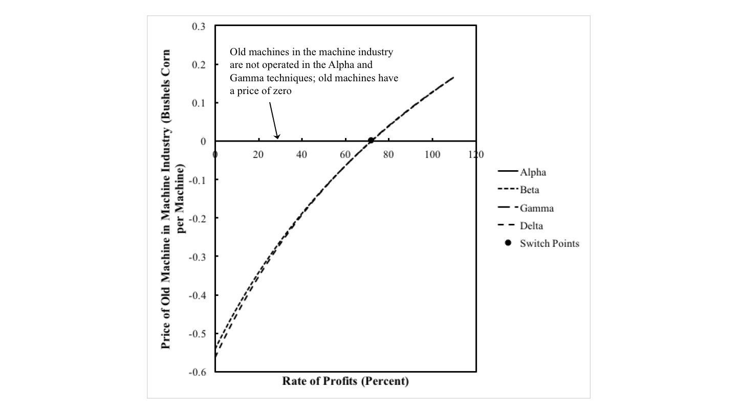
Next, I want to consider the price of an old machine in the machine sector. Figure 4 shows how the price of such a machine varies with the rate of profits for the price systems for each technique. An old machine is operated in the machine sector under the Beta and Delta techniques. For a rate of profits below the rate of profits at the switch point, the price of this old machine is negative. The implication is that the Beta and Delta techniques cannot be cost-minimizing in this range of the rate of profits. The old machine should not be operated for the second year; its economic life should be truncated. On the other hand, the price of an old machine is the machine industry is non-negative for a rate of profits larger than the rate of profits at the switch point, whatever the technique.

Figure 4: The Price of an Old Machine in the Machine Sector

Figure 5 graphs the price of an old machine in the corn sector. Such a machine is operated in this sector under the Gamma and Delta techniques. We have already seen that the Beta and Delta techniques cannot be cost-minimizing for a low rate of profits. The operation of an old machine in the corn sector should be truncated at a low rate of profits under the Gamma technique. So the condition that prices of old machines cannot be negative for the cost-minimizing technique implies that the Alpha technique is uniquely cost-minimizing at rates of profits smaller than the rate at the switch point.

Figure 5: The Price of an Old Machine in the Corn Sector

For high rates of profits, the use of an old machine in the corn sector must be truncated under the Delta technique. In fact, at Beta prices, the operation of an old machine in the corn sector incurs extra costs at high rates of profits. At Gamma prices, the operation of an old machine in the machine sector makes extra profits at high rates of profits. So from Figure 3, one knows that the Alpha technique is not cost-minimizing at high rates of profits. The Gamma technique cannot be cost-minimizing at high rates of profits, since a process (Process II) not in the technique makes extra profits. But by Figure 5, the Delta technique cannot be cost-minimizing at high rates of profits. Only the Beta technique is consistent with cost-minimization at high rates of profits.

So this analysis of the choice of technique based on which processes make extra profits, for each price system, and which prices of old machines are negative justifies, for this example, the results of an analysis based on the outer envelope for the wage curves for the various techniques.

5.0 Conclusion

I have briefly considered the effects of perturbations of a_{1, 4}. For a slightly higher value, the Alpha and Beta techniques, in order of an increasing rate of profits, are cost-minimizing. For a slightly lower value, the Alpha, Gamma, and Delta techniques are cost-minimizing. This fluke switch point arises as technical progresses leads it to be worthwhile to operate the machine for two years in the corn sector.

Nevertheless, am not sure if I fully understand how this fluke case fits into my taxonomy. Furthermore, I am seeking a numerical example with this fluke case in which a fuller perturbation analysis will find a case of capital-reversing, if not reswitching.

Sraffa's PoCbMoC At 60

Seminar

I finally watched Production of Commodities at 60. Our host and moderator is Matias Vernengo. Seminar participants are Franklin Serrano, Antonella Palumbo, and Ed Nell, who present in that order. They take questions at the end.

I cannot recall who made these points; they generally agreed. But here are some I noted. Sraffa is not only about an internal critique of marginalist theory, but a setting out of an alternative theory. This is a rediscovery of the classical theory of value.

Sraffa's theory is not restricted to perfect competition. Paul Sweezy was wrong to think that the advent of monopoly capitalism meant that only qualitative assertions could be made about value.

Ed Nell talks about linear programming, as contrasted to prices that support the reproduction of the economy. He is probably thinking of an appendix in Pasinetti (1977). I take his point, but I and others have shown that a LP can be used to formalize prices of reproduction.

In the Q and A at the end, Vernengo reads a question about whether Sraffa was inspired by Marx's schemes of simple and expanded reproduction in his development of his first and second system of equations equations. Like the seminar participants, I do not have a strong opinion on this question. I wish the scholars debating this would look into Sraffa's reading of the french translation of Kautsky's edition of Theories of Surplus Value. What is different about the later more complete edition? Does Sraffa's copy have marginal notes?

Another question concerns the relevance of steady state growth paths. Come to think of it, Serrano's remarks about a more general, looser concept might draw on his work on the supermultiplier, which he otherwise does not talk about. I think it was Nell who raises the point that Robinson did not think much of the analysis of the choice of technique. When one technique replaces another over historical time, this is not a choice with given knowledge of alternative techniques. What would Robinson think of my merging the two by considering, say, perturbations of coefficients of production in logical time? Probably not much.

Anyways, this is just a selection of topics from a far-ranging discussion.

Non-Uniform Rates Of Profits

This post presents a limited account of the history of analyzing prices of production with non-uniform rates of profits. I start from developments in post Sraffian price theory. D’Agata (2018) and Zambelli (2018b) have argued that Sraffian prices of production can still be defined when rates of profits have regular and persistent variations among industries. Barriers to entry or idiosyncratic properties of investment can result in such variations. Steedman (1981) presents the first formulation in post Sraffian price theory that I know of in English with systematic variations of the rate of profits among industries. Roemer (1981: 23-29) provides microfoundations for modeling imperfect competition in linear production models. He assumes different capitalists have different information sets; they only know of some of the production processes that are available. He argues that this can lead to specified ratios of rates of profits among industries. Cogliano et al. (2018) and Screpanti (2019) are some more Marxist contributions along the same lines.

Adam Smith (1776) called 'natural prices' what I, following Marx, am calling prices of production. He explained differences in rates of profits among industries as arising both in competitive conditions and as a result of barriers to entry. Book 1, Chapter X of The Wealth of Nations is titled 'Of wages and profits in the different employments of labour and stock'. According to Smith, the rate of profits is systematically higher in industries thought disagreeable or disgraceful. It is also higher in less risky investments, because capitalists overvalue their chance of gain and undervalue the chance of loss. (Smith also explained systematic differences in wages from these same causes. Typically, in my approach:

"We suppose labour to be uniform in quality or, what amounts to the same thing, we assume any differences in quality to have been previously reduced to equivalent differences in quantity so that each unit of labour receives the same wage" (Sraffa 1960: 11).))

Smith argues that for natural prices to obtain, employments must be well-known and long established in each neighborhood. Policy in European countries, according to Smith, restricted competition in some employments and encouraged excessive employments in others. Furthermore:

"It is to prevent this reduction of price, and consequently of wages and profit, by restraining that free competition..., that all corporations, and the greater part of corporation laws, have been established" (Smith 1776).

(This chapter contains another well-known quotation:

"People of the same trade seldom meet together, even for merriment and diversion, but the conversation ends in a conspiracy against the public, or in some contrivance to raise prices" (Smith 1776).)

David Ricardo and other classical economists accepted Smith’s account of the causes of non-uniform profits and wages.

Many groups of economists during the twentieth century developed theories of oligopoly and analyzed the effects on prices and the rate of profits of barriers to entry. Edward Chamberlin (1958) and Joan Robinson (1933) put forth almost simultaneously their theories of monopolistic and imperfect competition. Robinson drew on the earlier work of Sraffa (1926). These works clarified, to some extent, the assumptions needed for the neoclassical theory of perfect competition.

Some were inspired by empirical research. The Oxford Economists’ Research Group was set up in the 1930s. As part of the group’s research, Hall and Hitch (1939) found, in interviews with businessmen, that firms do not set prices based on marginal cost and marginal revenue. Michal Kalecki (1965) took these findings in stride and developed a theory of markup pricing as a microfoundation for his independently developed Keynesian macroeconomics. Perhaps some of my work can be seen as a partial answer to Steedman's questions for Kaleckians (Steedman 1992).

Old industrial organization, as developed by Joe Bain (1956) and Paolo Sylos Labini (1969), (Modigliani (1958) is a prescient survey.) rediscovered a classical notion of competition and a corresponding theory of oligopoly. Free competition is about the absence of barriers to entry, in contrast to the marginalist notion of perfect competition, in which managers of firms take prices as given.

Since I am interested in the labor theory of value, I want to mention the treatment of oligopoly and monopoly by economists associated with the Monthly Review. (For example, Sweezy (1942), Baran (1957), and Baran and Sweezy (1966).) As I read them, oligopolies and monopolies present a challenge to maintaining a quantitative theory of prices:

"Under conditions of monopoly, exchange ratios do not conform to labour-time ratios, nor do they stand in a theoretically demonstratable relation to labor-time ratios as is the case with prices of production." (Sweezy 1942: 270)

Baran (1957) is a Marxist who, as a consequence of his understanding of the importance of the role of monopoly, drops talk of 'surplus value' for the more qualitative concept of the 'surplus'. At the high level of abstraction of my work, however, this attitude seems unjustified.

Managerial theories of the firm (Marris (1964), Eichner (1973 and 1976), Harcourt and Kenyon (1976), and Wood (1975), for example. See also Penrose (1980).) were developed during the 1960s and 1970s. In these theories, firms set their markup over cost to generate internal funds to, in combination with external finance, fund investment plans to achieve a target rate of growth. They strive to achieve a normal rate of profits at a planned rate of capacity usage.

The research briefly summarized above has been quite influential, particularly among non-mainstream economists, to this day. For my purposes, I ignore distinctions among behavioral and managerial theories of the firm, administrated prices, full cost prices, normal cost prices, theories of the degree of monopoly, and markup pricing. (Lee (1999) emphasizes the distinctiveness of the theories of administered, normal cost, and markup price theories.) Rather, ratios of rates of profits among industries are taken as given parameters in defining prices of production.

This post is basically an abstract from something I may never publish.

Can We Hear Phil Mirowski In The Media Talk About Paul Milgrom And Robert Wilson?

The 2020 "Nobel Prize" in economics goes to Paul Milgrom and Robert Wilson. I suppose it is nice that economists acknowledge that markets are not natural entities but need to be constructed. For example, consider the Federal Communications Commission auction of the microwave spectrum.

The 2012 "Nobel Prize" went to Alvin Roth and Lloyd Shapley. The 1996 "Nobel Prize", to William Vickrey (a Post Keynesian, by the way) was also for acution theory. The 2002 prize went to Daniel Kahneman and Vernon Smith. Smith's work included experiments with markets constructed in the laboratory.

I do not know much about this field. But I am hoping some journalists know of Philip Mirowski, an expert on the history of information in economics, and get him to comment on the award this year.

A Fluke Case For Requirements For Use

Figure 1: Prices of Production

1.0 Introduction

This post presents a new kind of fluke case in the analysis of the choice of technique, at least new to me. I call this a pattern for requirements for use, and it can arise only in a case of joint production. My graphs in this post have some incomprehensible notation, since I am currently exploring perturbing parameters, in line with my research agenda. I know that perturbing the requirements for use removes the indeterminancy in this example.

2.0 The Givens

For this example, the data consist of the available technology and the proportions in which the two produced commodities, corn and silk, enter into the commodity basket specified by the requirements for use. I also choose a numeraire. The example is a perturbation of problem 8.2 in Kurz and Salvadori (1995).

Table 1 specifies a constant returns-to-scale technology. In each of three processes known to managers of firms at a given time, laborers work with inputs of corn and silk to produce outputs of corn, silk, or both. The inputs are completely used up in producing the output, and all three processes are assumed to take a year to complete. Since two commodities are produced in this numerical example, a technique consists of at most two processes. Table 2 lists the techniques and the processes corresponding to each technique.

Table 1: Coefficients of Production for The Technology

Input	Process
	I	II	III
Labor	1 Person-Yr.	1 Person-Yrs	(e/16) Person-Yr.
Corn	1 Bushel	1 Bushel	1 Bushel
Silk	1 Sq. Meter	1 Sq. Meter	1 Sq. Meter
Output
Corn	3 Bushels	5 Bushels	0 Bushel
Silk	3 Sq. Meters	0 Sq. Meter	5 Sq. Meters

Table 2: Techniques of Production

Technique	Proceses
Alpha	(I), (II)
Beta	(I), (III)
Gamma	(II), (III)
Delta	(I)
Epsilon	(II)
Zeta	(III)

The requirements for use are such that equal quantities of corn and silk are required. The numeraire consists of a commodity basket of one bushel corn and one square meter of silk.

3.0 Quantity Flows

Which techniques can satisfy the requirements for use? Suppose, contrary to the specification, that requirements for use specified that more bushels of corn be supplied than square meters of silk. The Alpha technique technique could satisfy these requirements for use, with Process I and Process II both being operated at a positive level of operations. As the requirements for corn declined, the relative level of operation of Process II would decline. The Alpha technique satisfies the given requirements for use with Process II operated at a level of zero. This is a corner case in which Process II still contributes an equation to the price system.

By a symmetric argument, the Beta technique can also satisfy the requirements for use. Process III is operated at a level of zero in the Beta techniquye.

The Gamma technique can satisfy any composition of the requirements of use, as in the theory of single production. So it can satisfy the requirements for use in this case, too.

The Delta technique can satisfy any requirements for use, as well. However, when the requirements for use specify an unequal number of bushels corn and square meters of silk, one commodity is in excess supply and its price of production is zero.

Neither the Epsilon nor the Zeta technique can satisfy the requirements for use when the net output must contain a positive quantity of both commodities.

4.0 Prices of Production

But being feasible, in the sense that a technique can satisfy the requirements for use, is not sufficient for a technique to be cost-minimizing. Prices of production must be considered, as in models of the production of commodities with single production. Prices of production vary with distribution and the technique. Figure 1, at the top of this post, graphs the price of corn for the three techniques which contribute two equations, in addition to the equation specifying the numeraire, to determine the four price variables (price of corn, price of silk, the wage, and the rate of profits).

4.1 The Alpha Technique

Suppose the Alpha technique is in operation. The wage can range from zero to two numeraire units per person-year. Figure 2 shows that the Alpha technique is not cost-minimizing at low rates of profits, but is cost-minimizing at high rates of profits. If, at low rates of profits, Process III replaces I, the Gamma technique will be adopted. If it replaces Process II, the Beta technique is adopted. But the Beta technique is not cost-minimizing at low rates of profits. (In a model of single production, it is unambiguous which process is replaced when a new process is introduced into a technique.)

Figure 2: Extra Profits with Prices for the Alpha Technique

4.2 The Beta Technique

On the contrary, suppose the Beta technique is in operation. Figure 3 shows that this technique is cost-minimizing only at high rates of profits. At low rates of profits, firms will have an incentive to operate Process II. If they replace Process III by Process II, firms will be operating the Alpha technique. The above analysis has shown that the Alpha technique would not be cost-minimizing in this range of the rate of profits. If Process I is replaced by Process II, firms would be operating the Gamma technique.

Figure 3: Extra Profits with Prices for the Beta Technique

4.3 The Gamma Technique

The Gamma technique is cost-minimizing at low rates of profits. Figure 4 shows extra profits for prices for the Gamma technique. Both the Alpha and the Beta technique are cost-minimizing at high rates of profits. Extra profits can be made in operating Process I at Gamma prices for high rates of profits. Firms would find it profitable to replace either Process III or Process II, resulting in either the Alpha or the Beta technique, respectively.

Figure 4: Extra Profits with Prices for the Gamma Technique

4.4 The Delta Technique

I am going to present the Delta technique in more detail. For Process I to neither make extra profits nor to incur extra costs, the following equality must obtain.

(p₁ + p₂)(1 + r) + w = 3 p₁ + 3 p₂

The specification of the numeraire yields the following equation:

p₁ + p₂ = 1

For the Delta technique to be cost-minimizing, the two equations above must hold, extra profits must not be obtainable in operating Process II, and extra profits must not be obtainable in operating Process III.

Prices drop out of the equation arising out of the requirement that Process I neither obtains extra profits nor incurrs extra costs. The wage is an affine function of the rate of profits:

w = 2 - r

The above wage curve is identical with the wage curves for the Alpha and the Beta techniques.

For the Delta technique to be cost-minimizing, firms must not be able to obtain extra profits in operating Process II. This condition yields an inequality:

p₁ ≤ 1 + r + w

Substituting the wage curve and re-arranging terms yields an upper bound on the price of corn:

p₁ ≤ 3/5

That is, the price of corn cannot exceed the price of corn falling out of the Alpha technique. This inequality is shown by the upper bound of the shaded region in Figure 1 at the top of this post.

The condition that firms cannot obtain extra profits in operating Process III also yields an inequality:

p₂ ≤ 1 + r + (e/16) w

Or the price of corn cannot fall below a lower bound:

(1/80)[64 - 2 e - (16 - e)r ≤ p₁

This inequality is shown by the lower bound of the shaded region in Figure 1.

The Delta technique can be consistent with cost-minimizing for any price of corn in the shaded region, including the boundaries. The two constraints combined impose a lower bound of the rate of profits:

[2 (8 - e)]/(16 - e) ≤ r

The lower bound on the rate of profits is the rate of profits at the switch point.

As with the Alpha, Beta, and Gamma techniques, one can plot extra profits versus the rate of profits for all processes, given the price system for the Delta technique. Since the Delta technique has an extra degree of freedom, one must choose a price, as well as, say, the rate of profits for such an analysis. Figure 5 shows such a graph for a price of corn of 3/5 numeraire units per bushel. The switch point here is at the same rate of profits as for the switch point shown in Figures 2 and 3. For rates of profits below the switch point, firms will want to adopt the Gamma technique. For rates of profits above the switch point, the Delta technique is cost-minimizing, but not uniquely so. Firms would also be willing to adopt the Alpha technique.

Figure 5: Extra Profits with One Set of Prices for Delta

But suppose the price of corn happens to be 1/2 numeraire units per bushel. Figure 6 plots extra profits in the three processes against the rate of profits. Firms will no longer be willing to choose to operate Process II along side Process I for some distribution of income. Costs exceed revenues for Process II, whatever the rate of profits.

Figure 6: Extra Profits with Another Set of Prices for Delta

For low rates of profits, the Delta technique is not cost-minimizing; firms will want to adopt the Beta technique. The "switch point" in Figure 6 is to the right of the switch point shown in all the other graphs in this post. From Figure 3, we know the adoption of the Beta technique is not the end of the story if the rate of profits lies below the rate of profits in the original switch point. For rates of profits between the two "switch points", prices must adjust until no extra profits can be obtained by operating the Beta technique. For rates of profits above the new "switch point", the Delta technique is uniquely cost minimizing at these prices and distribution of income. The Beta and Delta techniques are both cost-minimizing only at the new "switch point".

4.5 Summary

I find the possibilities in joint production confusing. I am fairly convinced of the above analysis, but I would not be surprised if my exposition could be improved. Anyway, here is a summary of the analysis of the choice of technique for this numerical example:

• When the rate of profits is smaller than the rate of profits at the switch point (or, equivalently, the wage is greater than the wage at the switch point), the Gamma technique is uniquely cost-minimizing. Prices are determined, given, say, the wage.
• When the rate of profits is larger than the rate of profits at the switch point (or the wage is lower than the wage at the switch point), the Alpha, Beta, and Delta techniques can all be cost-minimizing. Prices are indeterminate, with the price of corn confined to lie in the limits shown in Figure 1 by the curves for the Alpha and Beta techniques. Processes II and III in the technology are each operated at a level of zero, whatever the technique.
• When the rate of profits and the wage are as at the switch point, the Alpha, Beta, Gamma, or Delta technique are all cost-minimizing. Prices are determined, with a bushel corn priced at 3/5 numeraire units and a square meter of silk at 2/5 numeraire units.

5.0 Conclusion

This is a fluke case. If the proportions in which corn and silk enter into the commodity basket specified by requirements for use are varied at all, the indeterminancy of prices associated with a low wage vanishes. If bushels of corn exceeds square meters of silk in requirements for use, the Alpha and Gamma techniques are feasible. The Beta technique cannot satisfy the requirements for use. The Delta technique can satisfy the requirements for use, with an excess supply of silk at a price of zero. But then extra profits would be available by operating the second process. So only the Alpha or Gamma technique would be cost-minimizing, depending on income distribution.

Origins of Selection from the Prision Notebooks?

This is C27 in Sraffas archives.

97 Fortis Green
London N2
Tudor 0214

6th August 1966

Dear Piero,

I do not know whether you know Roger Simon, who is Secretary of the Labour Research Department. At all events he is a great admirer and enthusiast of Gramsci. Thanks to his initiative, plans are afoot (in which I too am collaborating) to publish a new volume of Gramsci's works translated into English and Lawrence & Wishart have agreed, in principle, to undertake publication.

We would very much welcome views and suggestions from you on how this should be done. The general idea at present is a bigger book than the L & W. 1957 translation (which is now out of print), including, if appropriate, passages already translated on that occasion. One line of thought that we are pursuing is that the volume should comprise mainly longer writings from the Notebooks and should be so presented that, if successful, it could be followed by further volumes, with the possible aim of ultimately translating all Gramsci's works. It would be good if the publication of this volume could sow the seeds of a growing interest in and knowledge of this outstanding political thinker, and so it is probably worth giving quite a bit of thought as to how this first step in that direction should be taken.

One problem is the choice of a translator; the ideal might be a young don specialising in twentieth century Italy and an admirer of Gramsci who would be keen to make a scholarly study of him, his times and his work. Do you know any such person?

Also do you by any chance know, or know anything of, Gwyn A. Williams who wrote a very interesting and scholarly article on Gramsci in the Journal of the History of Ideas, 1960, and who was at that time at the University College of Wales, Aberystwyth?

Are there other Gramsci scholars known to you?

I hope that we may have a chance of meeting some time in the Autumn.

With best wishes

Yours,

Stephen Bodington

Piero Sraffa Esq., M. A.,
Trinity College,
CAMBRIDGE.

Reference

• Antonio Gramsci (1971) Selections from the Prison Notebooks (Quintin Hoare and Geoffrey Nowell Smith ed. and trans.), London: Lawrence & Wishart

Keynes and Henderson Create A Qualitative Multiplier

In 1929, John Maynard Keynes and Hubert D. Henderson wrote, Can Lloyd George Do It? The Pledge Examined. This was published by The Nation and Athenaeum and is an examination of the pledge by the leader of the Liberal party, if elected, to dramatically reduce the amount of unemployment in Great Britain. (I was inspired to look up this work while reading Zachary Carter's new book.)

Chapter VI of Keynes and Henderson is concerned with "How Much Employment Will the Liberal Plan Provide?" The direct employment for each million pounds can be quantified. The authors divide the resulting indirect employment into two types. The first, in the industries that directly and indirectly supply road-building, housing, and so on, Keynes and Henderson think can be quantified:

VI.2 The Importance of Indirect Employment

"...There is nothing fanciful or fine-spun about the proposition that the construction of roads entails a demand for road materials, which entails a demand for labour and also for other commodities, which, in their turn, entail a demand for labour. Such reactions are of the very essence of the industrial process. Why, the first step towards a right understanding of the economic world is to realise how far-reaching such reactions are, to appreciate how vast is the range of trades and occupations which contribute to the production of the commonest commodities. That a demand for a suit of clothes implies a demand for yarns and tops, and so for wool; that the services of farmers, merchants, engineers, miners, transport workers, clerks, are all involved - this is the A B C of economic science...

Generally speaking, the indirect employment which schemes of capital expenditure would entail is far larger than the direct employment. This fact is one of the strongest arguments for pressing forward with such schemes; for it means that the greater part of the employment they would provide would be spread far and wide over the industries of the country. But the fact that the indirect employment would be spread far and wide does not mean that it is in the least doubtful or illusory. On the contrary, it is calculable within fairly precise limits..."

The second type of indirect employment results from the multiplier effects on aggregate demand of an increase in government spending. At this time, Keynes did not think these indirect effects could be estimated ahead of time, even though he considered them of immense importance:

VI.3 The Cumulative Force of Trade Activity

"But this is not the whole of the story. In addition to the indirect employment with which we have been dealing, a policy of development would promote employment in other ways. The fact that many workpeople who are now unemployed would be receiving wages instead of unemployment pay would mean an increase in effective purchasing power which would give a general stimulus to trade. Moreover, the greater trade activity would make for further trade activity; for the forces of prosperity, like those of trade depression, work with a cumulative effect. When trade is slack there is a tendency to postpone placing orders, a reluctance to lay in stocks, a general hesitation to go forward or to take risks. When, on the other hand, the wheels of trade begin to move briskly the opposite set of forces comes into play, a mood favourable to enterprise and capital spreads through the business community, and the expansion of trade gains accordingly a gathering momentum.

It is not possible to measure effects of this character with any sort of precision, and little or no account of them is, therefore, taken in 'We Can Conquer Unemployment." But, in our opinion, these effects are of immense importance. For this reason we believe that the effects on employment of a given capital expenditure would be far larger than the Liberal pamphlet assumes. These considerations have a bearing, it should be observed, on the time factor in Mr. Lloyd George's pledge. It is a mistake to suppose that a long interval would elapse after, let us say, the work of road construction had been commenced before the full effect on employment would be produced. In the the economic world, 'coming events cast their shadows before,' and the knowledge that large schemes of work were being undertaken would give an immediat fillip to the whole trade and industry of the country."

It would take the work, a few years later, of Richard Kahn and James Meade to formalize these indirect effects and show how to quantify them, in terms of the marginal propensity to consume.

"When Economists Are Wrong"

In a blog associated with the Frankfurter Allegmeine, Gerald Braunberger criticizes the effects of Sraffian political economy on Italian policy in the 1970s. I rely on google translate and subject matter expertise to make some sense out of this. By the way, Bertram Schefold shows up in the comments. I would like to know more about the motivations behind this. Does Braunberger think the public is increasingly aware that mainstream economics is broken?

Before I disagree, I note Braunberger seems well-informed on some points. I know of grumbles about Garegnani's treatment of Sraffa's archives. And I have heard that the Trieste summer schools were torn between those who emphasized long period logic and Post Keynesians who emphasized uncertainty, money, and historical time. On another point, I do not see why Sraffians giving policy advice should care about whether their advice is consistent with the advice Ricardo had for Britain during and after the Napoleonic war. I would think Sraffians in Italy during the 1970s would be more interested in Marx's views, anyways.

I do not understand what non-Sraffian theory Braunberger thinks exists. All economists should (but do not) recognize no reason exists to think that a lower real wage, in a time of depression, will encourage firms to adopt more labor-intensive techniques and thereby increase employment. In parallel, higher real wages need not decrease employment through the adoption of less labor-intensive techniques. Supply and demand just is not a logically-consistent model, in which conclusions follow from assumptions, of wages and employment.

This does not mean that real wages can be increased willy-nilly, without any consequences. Income effects could be important. And one might want to worry about the possibility of a capital strike. I agree that the political slogan, "The wage as the independent variable" draws directly on Sraffa.

More than economics was involved in the going-ons in Italy in the 1970s. When activists are kidnapping and executing the prime minister and the government is imprisioning leftists without discrimination, firms, government, and unions are unlikely to come to a peaceful agreement about distribution.

Furthermore, Italy was not isolated from the wider world. Were the lira and the mark pegged to the dollar before Nixon ended Bretton Woods? The world-wide rise in oil prices was not the result of Sraffian policy advice. Wage-push inflation arose in many countries; it was not just an Italian problem. Sraffa's colleagues had worked out an explanation of stagflation long before the event. I would think this is an example of when (heterodox) economists are right. (A Tax-based Income Policy (TIP) is a policy idea I associate with American Post Keynesians, like Sidney Weintraub, that might have been worth trying in some countries in the 1970s.)

Visualizing The Effects Of Markups: A Numeric Example

Figure 1: A Pattern Diagram

This post illustrates the numeric example used here. The example is of an economy in which two commodities, iron and corn, are produced by workers from inputs of iron and corn. Two processes are available for each industry, leading to a choice among four techniques. I analyze stationary states.

I look at prices of production, with a bushel corn as numeraire and wages paid out of the surplus at the end of the year. Prices of production are defined so as to allow for markups in both industries. Figure 1 shows the variation in switch points on the wage frontier with variations in the ratio of markups.

I am interested in how variations in markups can bring about qualitative changes favorable to labor pressing for higher wages. For example, around the switch point between Alpha and Gamma in Region 3 and at the lower wage for such a switch point in Region 4, a higher wage is associated with firms wanting to hire more workers, given the level of net output of corn.

Figure 2: The Solution of the LP in Region 1

I analyze the choice of technique by analyzing the solution of a linear program for a cost-minimizing firm. Figure 2 illustrates. (I have this figure wrong in my working paper.) Above the heavy locus, firms are willing to only produce iron. The regions in which profit-maximizing firms are willing to adopt each iron-producing process are indicated. Below the heavy locus, firms are only willing to produce corn. This region is also partitioned by the two corn-producing process.

Firms are willing to produce both iron and corn only along the heavy locus. The economy is capable of being reproduced only with the indicated combination of wages and prices. This is how the wage frontier appears in this space.

Figure 3: A Pattern over the Axis for the Scale Factor for the Rate of Profits

Figure 3 illustrates the solution to the LP with a higher markup in corn production or a smaller markup in iron production. For a wage of zero, firms are indifferent about the choice of the corn-producing process when prices are such that the economy can be reproduced. Figure 4 shows the case in which relative markups are such that firms are indifferent between the two iron-producing processes at a wage of zero.

Figure 4: Another Pattern over the Axis for the Scale Factor for the Rate of Profits

Figure 4 shows a curious case. Consider the point where firms are willing to operate the first iron-producing process and both of the corn-producing processes. At this combination of the wage and prices, firms are also willing to operate the second iron-producing process. This is a bit more obvious by examining Figures 5 and 6, which are for a slightly higher ratio of the markup in corn production to the markup in iron production. The region in which firms are willing to operate only the second iron-producing process has split up into three subregions. Figure 4 arises for a ratio of markups where the middle subregion is just emerging.

Figure 5: A Four-Technique Pattern

Figure 6: The Solution of the LP in Region 4

Figure 7: An Enlargement in Region 4

Figure 8 illustrates the ratio of markups in which the first and second of the three subregions, in which the firm is only willing to operate the second iron-producing processes are just merging. The middle subregion is such a sliver that it is not really visible on the graph.

Figure 8: A Reswitching Pattern

For the ratio of markups illustrated in Figure 9, firms are willing to operate the second-iron producing process all along the heavy locus. When prices are such that economy can be reproduced, they are willing to operate the first iron-producing process only at the indicated tangent point.

Figure 9: Another Reswitching Pattern

Figure 10 illustrates the solution to the LP for a ratio of markups in right-most region in Figure 1. Markups in the iron industry are much higher than the markups in the corn industry.

Figure 10: The Solution of the LP in Region 6

These diagrams illustrate, for a numerical example, the whole range of relative markups among industries. Qualitative changes in switch points are indicated. And I have demonstrated that the Cambridge capital controversy has implications for non-competitive markets. Can you find this point being made in the literature on industrial organization?

Visualizing the Effects of Markups on the Choice of Technique

I have a working paper.

Abstract: This article extends to unequal rates of profits a derivation of prices of production from a linear program. A partition of the price-wage space is illustrated in an example with two produced commodities. The variation in the solution of the LP with perturbations of relative markups is illustrated. This analysis provides an intuitive explanation of how the reswitching of techniques and of how capital reversing can emerge in non-competitive markets.

David Graeber (1961 - 2020) On Usenet A Long Time Ago

I first became aware of David Graeber as a poster on Usenet back in the 1990s.

Many people who have succeeded in this world have no interest in conducting honest discussions. I found some places where one could have cheerful talk, including with harsh disagreement. And I found other places not so much. I probably fit in with the latter.

Sometime in November 1998, a thread arose, "A Donaldism for David Friedman". David Friedman is Milton's son and also promotes plutocracy under the guise of 'liberty'. The thread was about how participants should treat other posters who continually lied and said others secretly wanted to set up a totalitarian dictatorship where they could kill those who disagreed with them. Graeber was not having any of this:

[Dan Clore wrote:]

David [Friedman] wrote:

His basic thesis is that most of the people who claim to be left anarchists are really leninists, or something similar, who mask their views because their true views are unfashionable. If he can demonstrate it about Chomsky, who has the virtue of having written lots of stuff over a long period of time, and if, by forcing people on line to defend Chomsky, he can demonstrate it about them, he can discredit (at least) online left-anarchism--as a movement, and perhaps as a theory. That tactic doesn't appear workable applied to you, since you seem to have no particular interest in defending Chomsky, but it might work for those who do. And, given his beliefs about left-anarchism, it seems to me that it is a reasonable tactic.

Unfortunately for Jimi's "basic thesis", Chomsky has a long historical record in print of attacking Marxism-Leninism and state socialism in general -- including the 1960s, when it was much, much more "fashionable" than anarchism / libertarian socialism. That fact that empirical evidence disproves Jimi's thesis only seems to make him believe in it all the more rabidly: draw what conclusions from that you will.

I am beginning to finally understand what Friedman means by "reasonable". He appears to apply the term only to whether one's actions are consistent with one's premises, and rational in the sense of logically coherent. He does not appear to feel that premises themselves can be unreasonable. One could presumably start from the assumption that David Friedman is indeed a purple-assed baboon and that he ate one's grandmother and as long as one's techniques of argument are consistent with this premise, one is not an unreasonable person.

The question is whether he realizes this  can only confuse everyone else because just about everyone else does not define "reasonable" in this  way. "Reasonable", for most people, implies among other things an ability to compromise, to accomodate other points of view... "Reasonable" implies you are _not_ a fanatic who starts with wild unfalsifiable accusations, not that you have correctly concluded that, if your opponents are evil monsters, then making wild unfalsifiable accusations is best way to make them look bad.

I put forward to Mr. Friedman, then: if you are really a reasonable person ("reasonable" in the common sense, not in your own specialized sense) you will stop using the word in this way because it is obviously deceptive. It allows you to constantly insist to people who do not know you are using the word in a highly idiosyncratic, specialized sense that obvious fanatics who never compromise on anything are "reasonable", and people who are not fanatics and interested in accomodating different points of view are not. At the very least you can shift to a word like "rational". "Reasonable" is an important word with a very rich history and your usage is, to my mind, and I think to others,  just a horrible  perversion of it.

DG

It is very difficult to navigate Google's version of the Usenet archives.

I thought Debt: The First 5,000 Years quite interesting. I probably recall it badly. I learned that money first emerged as the second-hand trading of promises in communities where everybody knew everybody. It was not a matter of solving a problem of the lack of the double-coincidence of wants in a barter system. These debts became more formal, more rigid, when communities became more hierarchical, more structured. The introduction of coins, as tokens, came about when you had outsiders, like an empire's soldiers visit, and they had no interest in participating in a village community as an equal. Debts periodically got out of hand, and a jubilee would be declared. (Yes, I know, Graeber was mistaken about Apple. I know several entrepreneurs who have started their own high tech companies.)

I was vaguely aware of Graeber jeopardizing his career at Yale with his support of the union for graduate students, his organizing role in Occupy Wall Street, and his move to London. I read his essay "Bullshit Jobs", but have yet to read the book.

This post is totally inadequate for an appreciation of him.

Update: Benjamin Balthaser in Jacobin, Michael Hardt in Jacobin, Malcolm Harris in the Nation, Sam Roberts for the New York Times, Nathan Robinson in his Current Affairs, Rebeccca Solnit in the Guardian, and many in the New York Review of Books.

A Derivation Of Sraffa's First Equations

1.0 Introduction

Piero Sraffa wrote down his 'first equations' in 1927, for an economy without a surplus. D3/12/5 starts with these equations for an economy with three produced commodities. I always thought that they did not make dimensional sense, but Garegnani (2005) argues otherwise. This post details Garegnani's argument, albeit with my own notation.

There are arguments about how and why Sraffa started on his research project I do not address here. The question is how did he relate what he was doing at this early date to Marx. In addition to Garegnani, DeVivo, Gehrke, Gilibert, Kurz, and Salvadori are worth reading here.

2.0 Givens

I assume an economy in a self-replacing state in which n + 1 commodities are produced.

• c_0,0 is the input of the first commodity used in producing the output of the first industry.
• (c_{., 0})^T = [c_1,0, c_2,0, ..., c_n,0] are the inputs of the remaining n commodities used in producing the output of first industry.
• c₀ = [c_0,1, c_0,2, ..., c_0,n] are the inputs of the first commodity used in producing the output of the remaining industries
• The element c_i,j, i, j = 1, 2, ..., n, of the matrix C is the input of the ith commodity used in producing the output of the jth industry.
• q₀ = is the quantity produced of the first commodity.
• (q)^T = [q₁, q₂, ..., c_n] are the outputs of the remaining n commodities used in producing the output of first industry.

All quantities are given in physical units. I abstract from fixed capital; all inputs are used up in the production of the outputs. Table 1 presents these parameters for the first example in the first chapter in Sraffa 1960.

Table 1: The Example from Sraffa (1960), Chapter 1

Input	Industry
	Iron	Wheat
Iron	c0, 0 = 8 tons iron	c0 = [12 tons iron]
Wheat	c., 0 = [120 quarters wheat]	C = [280 quarters wheat]
Output	q0 = 20 tons iron	q = [400 quarters wheat]

The following must hold for economy to be in a self-replacing state:

q_i = c_i,0 + c_i,1 + ... + c_i,n, i = 0, 2, ..., n

All quantities are non-negative. The economy must hang together in some sense. In Sraffa's terminology, all commodities are basic.

3.0 Coefficients of Production

I like to think of the coefficients scaled for unit output in each industry. Accordingly, define:

a_{0, 0} = c_{0, 0}/q₀

(a_{., 0})_i = (c_{., 0})_i/q_j, i = 1, 2, ..., n

(a₀)_j = (c₀)_j/q_j, j = 1, 2, ..., n

(A)_i,j = (C)_i,j/q_j, i, j = 1, 2, ..., n

4.0 All Quantities Measured in Unit Outputs of the First Industry

The given inputs can be thought of as produced in the previous year. The amount of, say, iron directly used as input in producing other commodities is (a₀ q). Table 2 indicates how much iron is needed as input in all previous years.

Table 2: Iron Inputs for Other Commodities

Year	Iron
0	a0 q
1	a0 A q
2	a0 (A)2q
...	...
n	a0 (A)nq
...	...

Even though my notation picks out the first commodity, there is nothing special about it. Suppose some commodity is selected. Let v₀ be the quantity of this commodity needed directly and indirectly to produce a unit of the first commodity. Let v be the quantities of this commodity needed directly and indirectly to produce each of the remaining commodities. v₀ and v must satisfy the following system of n + 1 linear equations:

v₀ a_{0, 0} + v a_{., 0} = v₀

v₀ a₀ + v A = v

For a non-trivial solution to exist, the determinant of the matrix in Table 3 must be zero, which it is in the case pf the Sraffa example.

Table 3: A Matrix

1 - a0, 0 = (3/5) tons	-a0 = [(-3/100) tons]
-a., 0 = [-6 quarters]	I - A = [(3/10) quarters]

I set v₀ to unity. The amount of this commodity used directly and indirectly in the production of all other commodities is easily found:

v = a₀(I - A)^-1

5.0 Rescaling the Givens

I then rescale the givens.

b_{0, 0} = v₀ c_{0, 0}

b_{i, 0} = v_i (c_{., 0})_i, i = 1, 2, ..., n

b_{0, j} = v₀ (c₀)_j, j = 1, 2, ..., n

b_{i, j} = v_i c_{i, j}, i, j = 1, 2, ..., n

s₀ = v₀ q₀

s_i = v_i q_i, i = 1, 2, ..., n

Table 4 presents Sraffa's example with these calculations. Here, a unit of wheat is 10 quarters. That is, one ton iron is used directly and indirectly in producing 10 quarters of wheat.

Table 4: Sraffa's Example Again

Input	Industry
	Iron	Wheat
Iron	b0, 0 = 8 tons iron	b0 = [12 tons iron]
Wheat	b., 0 = [12 tons wheat]	B = [28 tons wheat]
Output	s0 = 20 tons iron	s = [40 tons wheat]

I then have Sraffa's 'first equations':

b_{0, j} + b_{1, j} + ... + b_{n, j} = s_j, j = 0, 1, ..., n

For the economy to be in a self-replacing state, the following must hold:

b_{i, 0} + b_{i, 1} + ... + b_{i, n} = s_i, i = 0, 1, ..., n

Even though I am adding together, say, quantities of iron and wheat, the dimensions are consistent.

6.0 A Re-interpretation

Suppose the first produced commodity is labor, not iron. c_{0, 0} becomes the amount of labor performed in households (outside the market) to reproduce the labor force. c_{., 0} is the commodity basket paid out in wages when the workers obtain all of the surplus product. a₀ are the direct labor coefficients for each industry, and A is the Leontief input-output matrix. v is the vector of labor valus (also known as employment multipliers). Under the assumptions, prices of production are identical to labor values.

This model is descriptive. The givens do not show how required inputs might decrease with innovation or the formal and real subsumption of labor.

References

• Garegnani, Pierangelo (2005) On a turning point in Sraffa's theoretic and interpretative position in the late 1920s. European Journal of the History of Economic Thouht 12 (3): 453-492.
• Gehrke, Christian, Heinz D. Kurz, and Neri Salvadori (2019) On the 'origins' of Sraffa's production equations: A reply to de Vivo. Review of Ploitical Economy 31 (1): 100-114.