|
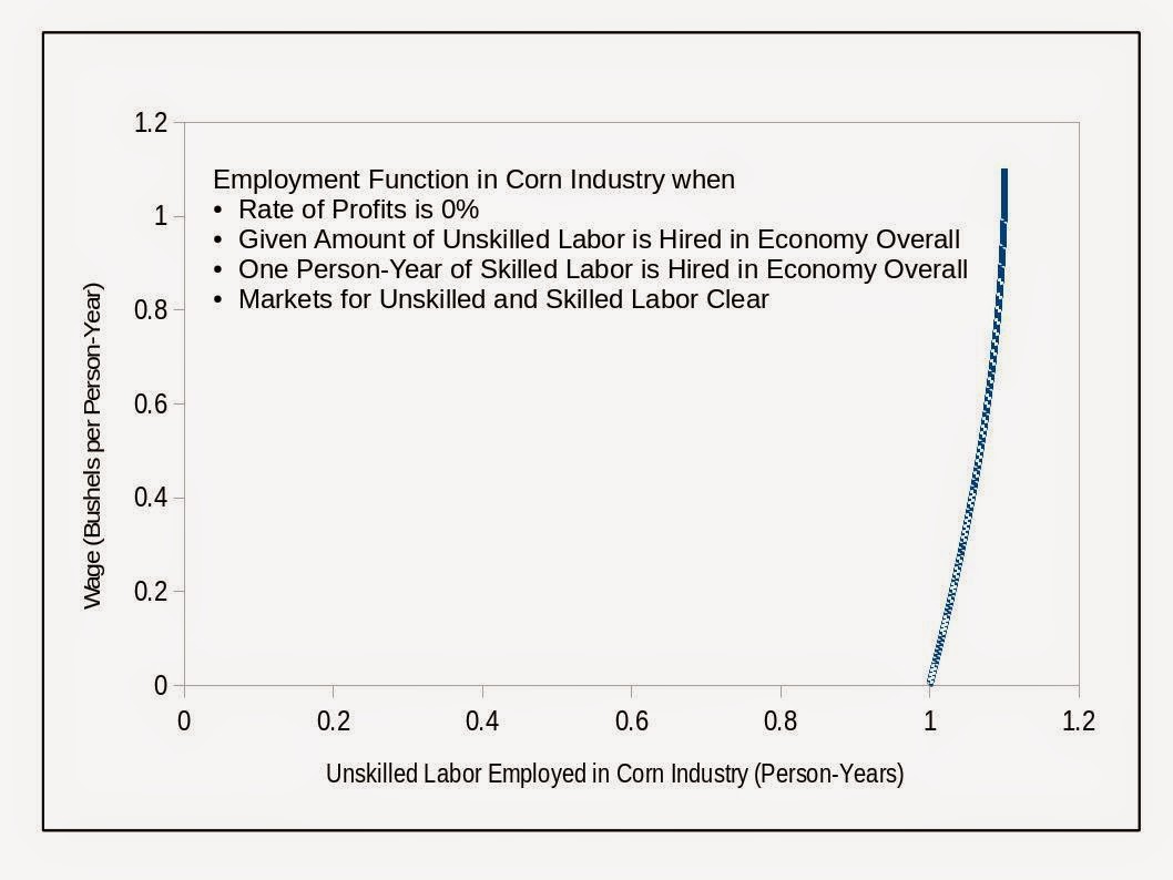
| Figure 1: "Labor Demand" in the Consumer Goods Industry |
In this post, I work through an example created by Arrigo Opocher and Ian Steedman. In this example, circulating capital is represented by machines of one of a continuum of types, and I compare stationary states. Unskilled and skilled workers use the machines to produce corn, along with more machines. The output of machines are needed to sustain production in future periods. In the stationary states, the same rate of profits is earned in all industries with a positive output. In fact, only the special case when the rate of profits is zero is considered here.
The (slice of) the so-called factor price frontier in this example resembles Paul Samuelson's surrogate production function. Aggregate relationships in this example are "non-perverse". In other words, they do not violate the outdated and exploded intuition of neoclassical microeconomics. The aggregate production function shows positive, but diminishing, marginal returns, in the relevant range, to inputs of factors of production. Lower wages for unskilled labor are associated with capitalists desiring to employ more unskilled labor in the economy overall.
But a perverse relationship arises in the market for corn. Corn is the only consumer good in the example. If capitalists are to want to employ more unskilled labor directly in the production of corn, the wage for unskilled labor must be higher, not lower (Figure 1). If more unskilled labor is available for production, and markets clear, more corn is produced. But when capitalists choose the cost-minimizing technology, at prices and wages they take as given, the quantity of unskilled labor used as input, in the corn industry, per bushel corn produced, decreases. This decrease overwhelms the increased output of corn, and the employment of unskilled labor in the corn industry declines.
2.0 The TechnologyConsider a simple capitalist economy, composed of (unskilled and skilled) workers and capitalists. After replacing (circulating) capital goods, output consists of a single consumption good, corn. Unskilled workers are paid the wage w, and skilled workers are paid the wage W out of the harvest. Both wages are in units of bushels corn per person year. Capitalists obtain the rate of profits r. The technology consists of an infinite number of Constant-Returns-to-Scale (CRS) techniques, indexed by s. Table 1 presents the coefficients of production for a single technique.
| Inputs | Machine Industry | Corn Industry |
| Unskilled Labor | a(s) l(s) Person-Years | l(s) Person-Years |
| Skilled Labor | a(s) t(s) Person-Year | t(s) Person-Years |
| Machines | a(s) Machines | 1 Machine |
| Outputs | 1 Machine | 1 Bushel Corn |
Notice that the first column of inputs in Table 1 is proportional to - that is, a constant multiple of the - second column. This is akin to Karl Marx's assumption of a constant Organic Composition of Capital, an unrealistic assumption that simplifies price theory.
The index s for the technology is chosen from a set of real numbers, with √ 6 ≤ s ≤ 3. The parameters of a technique are defined in terms of the index as follows:
a(s) = 2 - (6/s) + (6/s2)
l(s) = 1/s
t(s) = 1/s2
Each different value of the index s is associated with the use of a different type of machine. And different quantites of unskilled and skilled labor must be used with each different type of machine to produce the output.
I compare stationary states under these assumptions:
- L person-years of unskilled labor are available for employment in the economy, with √ 6 ≤ L ≤ 3.
- T = 1 person-years of skilled labor are available for employment in the economy.
- r = 0% is the rate of profits in the stationary states considered here.
- The markets for skilled and unskilled labor both clear.
- The production of machines and corn are adapted to a stationary state. So the endowments of machines (by type) are found by solving the model, not givens.
Given the type of machine, suppose the quantity of corn, c(s), produced is:
c(s) = [1 - a(s)]/t(s) = s2 [1 - a(s)]
Let the number of machines, m(s), produced be:
m(s) = 1/t(s) = s2
Table 2 shows the output of the machine and corn industries, scaled to produce these gross outputs.
| Inputs | Machine Industry | Corn Industry |
| Unskilled Labor | s a(s) Person-Years | s [1 - a(s)] Person-Years |
| Skilled Labor | a(s) Person-Year | [1 - a(s)] Person-Years |
| Machines | s2 a(s) Machines | s2 [1 - a(s)] Machines |
| Outputs | m(s) Machines | c(s) Bushels Corn |
For these quantity flows, the total employment of unskilled labor is s. The total employment of skilled labor is one person-year. The total inputs of machines, which are used up each year, are replaced by the output of the machine industry.
4.0 Stationary State Prices in the Special CaseSection 3 specifies quantity flows in a stationary state, given the type of machine. The capitalists choose the technique, including the machine, based on price. Let corn be numeraire, and suppose workers are paid at the end of the production period. If the same rate of profits is earned in the production of machines and corn, the following pair of equations must be satisfied for the technique in use:
p a(s)(1 + r) + a(s) l(s) w + a(s) t(s) W = p
p(1 + r) + l(s) w + t(s) W = 1
These equations have two degrees of freedom. One is eliminated by only considering the special case in which the rate of profits is zero. The other can be seen by expressing the solution as a function of, say, the wage for unskilled labor. In this sense, the solution of the system of equations for prices in a stationary state, given the special case assumption and the technique, is:
p = a(s)
W = [1 - a(s) - l(s) w]/t(s)
Or:
p = 2 - (6/s) + (6/s2)
W = - s2 + s(6 - w) - 6
The wage of skilled labor, given the technique, is an affine function of the wage of unskilled labor. Figure 2 illustrates this function for three different techniques. This figure is akin to Figure 2b on page 197 of Samuelson (1962), which shows how to construct the so-called factor price frontier for Samuelson's surrogate production function.

|
| Figure 2: Wage-Wage Curves |
In a stationary state, capitalists will have adopted the cost-minimizing technique. The cost-minimizing technique, given the wage of unskilled labor, corresponds to the technique on the outer envelope (that is, the frontier) formed from all (uncountably infinite) functions that one might plot in Figure 2. One can find the technique on the frontier by setting the derivative, with respect to the index s, of the wage-wage curve equal to zero:
dW/ds = 0
Thus, the machine type used by the cost-minimizing technique, in this special case, is the following function of the wage of unskilled labor:
s = (6 - w)/2
The frontier has the equation:
W = (1/4)w2 - 3 w + 3
The wage, w, of skilled labor ranges from 0 to (6 - 2 √ 6 ). The wage of skilled labor, W, ranges from 0 to 3. If the rate of profits were positive, the wage-wage frontier would lie inside the frontier found here.
5.0 Some Aggregate MarketsThe results found so far can be combined.
5.1 The Market for Unskilled LaborI have postulated that L person-years of unskilled labor and one person-year of skilled labor are available for employment in a stationary state. For quantity flows in a stationary state to fully employ both types of labor, the index for the machine type must be:
s = L
For this machine type to correspond to the cost-minimizing technique, given a rate of profits of zero and market clearing for both labor markets, the wage of unskilled labor must be the following function of unskilled labor:
w = 6 - 2 L
Figure 3 plots the wage for unskilled labor, under these assumptions, with the amount of unskilled labor firms want to hire in a stationary state. In this example, for more unskilled labor to be hired in a stationary state, its real wage must be lower. This property is particular to this example; it does not generalize.
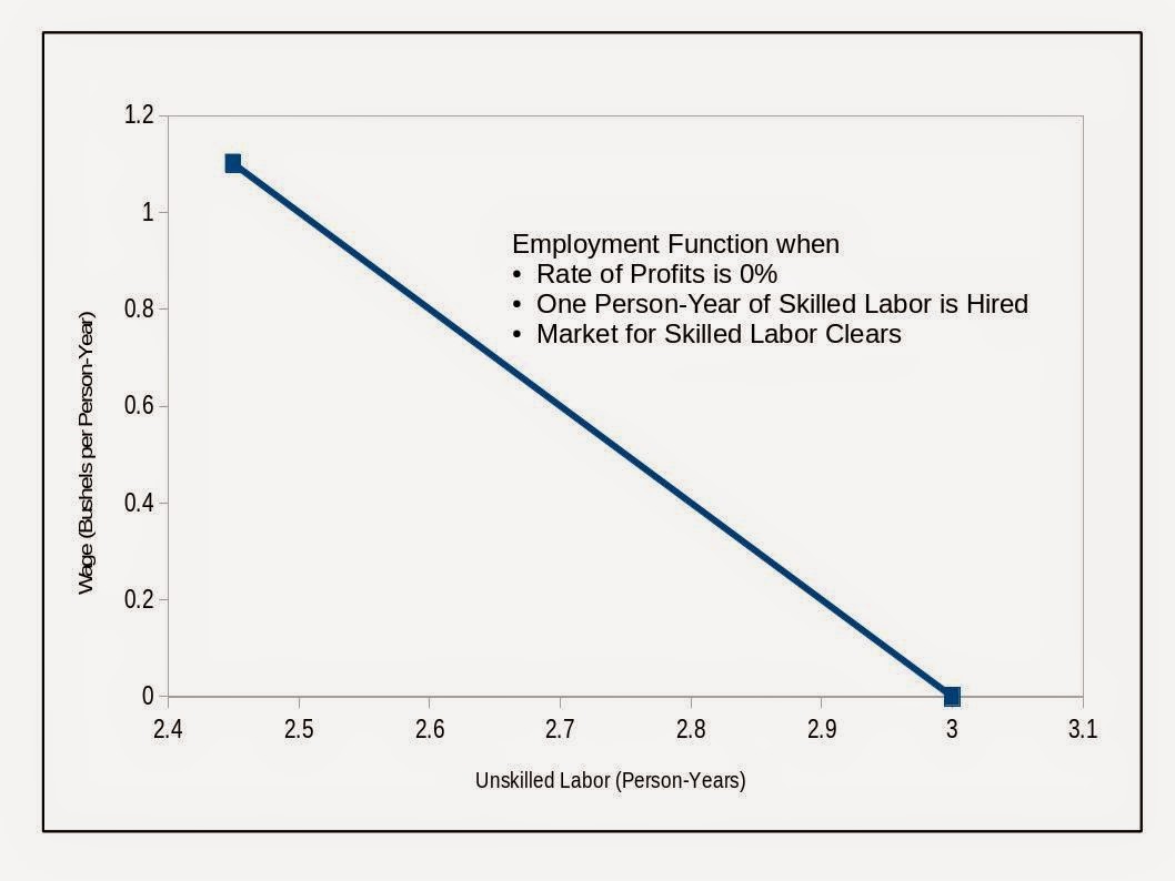
|
| Figure 3: Employment of Unskilled Labor |
The analysis so far has shown how to determine the cost minimizing technique and the wage for unskilled labor as a function of the amount of unskilled labor employed in a stationary state. And the wage for skilled labor is a function of the wage for unskilled labor, as shown by the wage-wage frontier. The wage for skilled labor can accordingly be expressed as a function of the amount of unskilled labor employed in a stationary state.
W = L2 - 6
Figure 4 shows the wage of skilled labor plotted against the quantity of skilled labor firms desire to hire in this example. In some sense, this function neither slopes up nor down.

|
| Figure 4: Employment of Skilled Labor |
Under the above assumptions, one can find the type and number of machines, m(s), produced in a stationary state. For stationary states in which different quantities of unskilled labor are employed, different types of machines will be produced. Quantities of different types of machines are incommensurable; physical measures of different types of capital cannot be plotted together on the same axis. A numeraire measure of the quantity of capital, k, can be found by taking the product of the price of machines and their physical quantity:
K = p m(s) = a(s) m(s)
Under the assumption that markets for unskilled and skilled labor clear, one can express numeraire units of capital as a function of the person-years of unskilled labor employed in a stationary state.
K = 2(L2 - 3 L + 3)
Figure 5 shows the rate of profits plotted against the above quantity of capital. In this special case, the rate of profits of capital is a non-increasing function of the quantity of capital.

|
| Figure 5: Value of Capital |
The previous section shows that no phenomena that violates outdated neoclassical price theory arises in aggregate markets for unskilled labor, skilled labor, or capital, in this particular example. But consider how much unskilled labor firms, under these assumptions, want to employ in the production of corn. Figure 1 shows the graph of the wage, w, for unskilled labor against the unskilled labor, l2, hired in the production of corn. That function can be found as:
l2 = (-L2 + 6 L - 6)/L
And this function slopes up, contrary to what neoclassical economists would have expected about half a century ago.
7.0 ConclusionIf you work through enough examples in production theory, you ought to conclude that it is hard to find any justification for mainstream theories in microeconomics. Why so many economists continue to teach archaic balderdash, and (mis)train their intuition accordingly, is a question.
References- Arrigo Opocher and Ian Steedman (2013). Unconventional results with surrogate production functions Global and Local Economic Review, V. 17, No. 1: pp. 45-53.
- Paul A. Samuelson (1962). Parable and realism in capital theory: The surrogate production function, Review of Economic Studies, V. 29, No. 3: pp. 193-206.


No comments:
Post a Comment