On the Gain and Loss from Trade

I have written up my recent explorations in the theory of international trade.

Abstract: This article considers a model of international trade in which the number of produced commodities does not exceed the number of countries engaged in trade. Technology is modeled such that each commodity can be produced in each country from a finite series of dated labor inputs. The existence of a positive rate of profits may lead a country to specialize differently than how it would with a zero rate of profits. Trade may leave consumers in a country worse off, as compared with autarky, when the rate of profits is positive. The existence of more than two countries provides a possibility that the Production Possibilities Frontier (PPF) with trade is neither unambiguously above or below the PPF under autarky. This article re-iterates, in a setting with more than two produced commodities and more than two countries, demonstrations that the argument for free trade is logically invalid, given positive rates of profits.

Elsewhere

• Howard Reed argues we should rip up textbooks for mainstream economics and start over. (Some of what he says echoes an argument of mine.)
• I do not think Diane Coyle addresses Reed's points.
• Cahal Moran argues the problem is economics, not economists.
• Beatrice Cherrier has some frankly speculative posts on what limitations economists accepted in emphasizing tractability in developing models.
• Nathan Robinson does not like the word "neoliberalism", but understands there is a point to using it.
• David Glasner writes about Hayek's introduction of the theory of intertemporal and temporary equilibrium paths into economics. (I have no problem for those who look for Irving Fisher as a precursor of for more-or-less simultaneous discoveries in Sweden.)

Class Struggle And Specialization In International Trade

This post continues a previous numeric example. The firms in each of three countries are assumed to know a technology for producing corn, wine, and linen. The technology is such that each commodity can be produced in each country. The technology varies among countries.

Each of these small open economies can specialize and obtain non-produced commodities through foreign trade. I confine myself to patterns of specialization in which:

• Each country produces exactly one commodity domestically.
• Each commodity is produced in one country.

Six patterns of specializations meet these criteria. Table 1 lists the commodity produced in each country for each pattern of specialization.

Table 1: Patterns of Specialization

	England	Portugal	Germany
I	Corn	Wine	Linen
II	Corn	Linen	Wine
III	Wine	Corn	Linen
IV	Wine	Linen	Corn
V	Linen	Corn	Wine
V	Linen	Wine	Corn

I have found out that, in my example, each specialization is consistent with a long period position. I take the international price of corn as numeraire. That is, p₁ = 1. Table 2 lists the prices of the other commodities, p₂ and p₃, that are traded domestically. It also lists rates of profits, r₁, r₂, and r₃, in each country. This data is sufficient to calculate the wage in each country. The wage is such that supernormal profits are not earned in the commodity produced domestically, but the cost (including profits) does not exceed revenues for produced commodities. With these wages, the costs of producing a commodity in which a country does not specialize will exceed the price. It is cheaper in each country to acquire such commodities on international markets.

Table 2: International Prices and Rates of Profits

	Price of Wine	Price of Linen	Rate of Profits
			England	Portugal	Germany
I	3/4	2/3	0%	0%	0%
II	0.83	0.7	50%	0%	20%
III	0.883	3/4	20%	60%	0%
IV	1.06	1.3	60%	50%	90%
V	1.1	5/4	40%	150%	70%
VI	4/5	0.754	0%	20%	20%

The prices shown in Table 2 are not unique. For the given set of rates of profits, international prices must fall within a certain range to obtain a long period position consistent with the pattern of specialization. And rates of profits may vary in certain ranges too. I have not figured out a good way of visualizing how the spaces of prices and rates of profits is divided up by the patterns of specialization. Maybe a region for a given pattern of specialization if, contrary to this example, restitching was possible under autarky.

The numeric example illustrates that:

• The pattern of specialization in foreign trade can be driven by technology and the distribution of income.
• Only some distributions are compatible with all countries being able to specialize in a consistent way.
• The results of such specialization may not provide a country with overall gains from trade, nevermind individual groups defined by the functional distribution of income.

I have assumed constant returns to scale, but which commodity a country specializes in producing may be of importance because of considerations of learning-by-doing. Technological progress may be easier to obtain in some commodities (e.g., manufactured industrial products) than others (e.g., products of agriculture). I suspect these observations generalize to a more comprehensive Neo-Ricardian theory of trade, such as that of Yoshinori Shiozawa.

These theoretical observations, I guess, are enough to blow up much mainstream teaching on trade. I might have even made some progress on the work of Mainwaring, Metcalfe, and Steedman. Nevertheless, this model puts much aside. I am thinking of, especially, Keynesian issues of exports, imports, and effective demand; foreign exchange rates and monetary policy; and international finance.

The Gain And Loss From Trade: More On A Numeric Example

Figure 1: The Production Possibility Frontier, With And Without Trade, In "Germany"

1.0 Introduction

I continue to blunder around in parameter space in exploring my numeric example in the previous post. In this post, I continue to adopt the same assumptions for a model of three countries engaged in international trade with three produced commodities. In particular, workers are assumed to be unable to immigrate, capitalists only invest in their own country, and produced means of production are not traded. Thus, wage rates and rates of profits may vary among countries, with no tendency to change or approach equality.

2.0 Outline of the Model

For this intellectual exercise, I make the same assumptions about technology, available in each country, but differing among them. Corn, wine, and linen can each be produced from a dated series of labor inputs. Under the restrictive assumptions illustrated by the numeric example, one can rank commodities by how labor-intensive they are. Corn is most labor-intensive, and linen is least. Wine is of an intermediate labor-intensive. The endowment of labor is also taken as given.

The rate of profits is taken as given in each country. One then wants to find a set of international prices for corn, wine, and linen such that a pattern of specialization can arise for the given data. Under a model of small, open economies, the firms in each country take prices as given. In such specialization, each country will specialize in producing at least one commodity, and each commodity will be produced in one or another country. The wage in each country will be such that no pure economic profits (also known as supernormal profits) will be earned in the production of any commodities. And costs, including charges for the prevailing rate of profits, will exceed the price of all commodities that firms in each country are unwilling to produce.

3.0 Countries Specializing in Producing One Commodity

Table 1 exhibits a set of prices, for the given rates of profits, that meets these conditions. Each country specializes in the production of one commodity. England produces linen, Portugal produces corn, and Germany produces wine. The wages in each country are as shown.

Table 1: Prices with Trade

Commodity	England	Portugal	Germany
Corn	p1 = 3240/11
Wine	p2 = 324
Linen	p3 = 4050/11
Rate of Profits	r1 = 2/5	r2 = 3/2	r3 = 7/10
Wage	w1 = 4050/1199	w2 = 162/121	w3 = 1

For this particular set of prices, each country specializes differently than they would if the rates of profits were zero in each country. And they specialize differently than they would at the prices and positive rates of profits in my previous exploration of this example.

4.0 Production Possibility Frontiers (PPFs)

In the textbook theory of comparative advantage, an unambiguous gain from trade is shown by comparing the Production Possibilities Frontier (PPF) with trade and under autarky. The claim is that the with-trade PPF is moved outward from what it would be under autarky. If the consumption basket contains any commodities that must be bought on international markets, the with-trade equilibrium is supposedly unambiguously better for the country. No commodity must be consumed in a smaller amount than under autarky, and some commodities can be produced in larger quantities. Some may be hurt by trade, perhaps because they receive profits from industries whose domestic production has been replaced by imports. But they could be compensated out of the increased consumption basket, while still leaving everybody else better off in the country under consideration.

To check the textbook argument, one would look at the PPFs in each of England, Portugal, and Germany. And the textbook story is validated for England in this numeric example, with these prices and pattern of specialization. The PPF for England is rotated outwards, as compared with autarky. They coincide at the intersection with the linen axis. For every other consumption basket with non-negative quantities, the English with-trade PPF lies outside the autarkic PPF. England gains from trade.

The with-trade and autarkic PPFs for Portugal (Figure 2) replicate my previous finding that specialization can result in a loss from trade. The argument from comparative advantage is logically invalid, given positive rates of profits among countries engaged in international trade. The with-trade PPF in Portugal is rotated inwards. Portugal is unambiguously worse off with trade.

Figure 2: The Production Possibility Frontier, With And Without Trade, In "Portugal"

The story from Germany illustrates a possibility that cannot arise in the two-country, two-commodity model. The with-trade PPF (Figure 1) is neither rotated outwards nor inwards, as compared with the autarkic PPF. Along one dimension (linen), the with-trade PPF lies outside the autarkic PPF. Along another dimension (corn), it lies inside the autarkic PPF. Whether Germany is worse or better off with-trade depends on the composition of the commodity basket.

5.0 Remarks on Krugman and Obstfeld

I am unsure what I think of Krugman and Obstfeld, so far. Chapter 2 presents the argument from comparative advantage. They hammer home that, in the Ricardian model, countries are better off with-trade, no question about it. In this chapter, inputs consist only of labor, and no profits are earned. I do not know that they are clear that labor inputs are only direct. (In my example, I have labor inputs distributed over time, thereby providing a role for a rate of profits.)

In Chapter 3, they have manufacturing goods produced from labor and capital, as specified by a production function. I am not sure they ever take the marginal product of capital. They show output as a function of labor, with a diminishing marginal product. Although they do have some remarks on the supply of labor, they seem to be considering a medium term model where manufacturing output is produced with given technical conditions and a given set of production facilities. The point is to show that trade has impacts on the distribution of income in a country and can hurt some, if they are not compensated out of the supposed gains.

Chapter 4 sets out the Heckscher-Ohlin-Samuelson model in the two-factor, two-country, two-commodity case. The factors are labeled labor and land. This is as far as I've gotten in my reading.

One reading of the above is that Krugman and Obstfeld are carefully working around the Cambridge Capital Controversy. I do not know that they entirely succeed in Chapter 3. Their chapters have points, and I, of course, question their Chapter 2 claim that the gains of trade are unambiguously positive. Presumably, they would point to later chapters that put forth qualifications about imperfect competition and increasing returns to scale - a textbook presentation of the work that won Krugman a Nobel prize. Or they might point to a need in pedagogy to drum home simple points. Furthermore, their textbook, they could argues, teaches what (mainstream) economists have settled on as a consensus of what international economics is.

But what happens when the consensus has been shown to be simply wrong almost half a century ago? I know I have previously thought Krugman's offhand remarks on his blog about the CCC did not seem particularly informed. Has he ever referenced, say, Ian Steedman, in his academic work?

References

• Paul R. Krugman and Maurice Obstfeld (2003). International Economics: Theory and Policy, sixth edition.

The Loss From Trade: A Numeric Example With Three Countries And Three Produced Commodities

Figure 1: The Production Possibility Frontier, With And Without Trade, In "Germany"

1.0 Introduction

This post presents a numeric example of a Ricardian model of small, open economies engaged in trade. Each of three countries specializes in producing one of three commodities. Technology is modeled following an Austrian approach. Each commodity can be produced in each country from inputs of labor and "capital". Endowments of labor are taken as given parameters. It makes no sense to take the endowment of capital as a given parameter.

The with-trade Production Possibilities Frontier (PPF) can be compared to the autarkic PPF in each of the three countries. And it is unambiguously rotated inwards in one country for the set of international prices and rates of profits I consider. One cannot correctly conclude, in the traditional textbook approach, that free trade makes the inhabitants of a country better off in the aggregate.

I have previously written up an analogous argument in the two-commodity, two-country case. I should have cited Steedman and Metcalfe (1973). If I had, I would have known that my originality was less than I suggested. Shiozawa argues convincingly that the sort of model illustrated in this post can only be offered as an intellectual exercise. A more empirically applicable model would have trade in intermediate products, and the number of traded commodities would exceed the number of countries. On the other hand, I do not know of any comparable write-up of an example with three or more commodities and countries, as here.

2.0 Assumptions

Consider a model of three countries - England, Portugal, and Germany - in which three commodities are potentially traded on international markets by each country.

• Each country can produce any of the three commodities.
• The managers of firms in each country know a given flow input-point output technology with the structure described in Section 3. The technology differs among countries.
• Each country has a given endowment of labor, the only non-produced factor of production in each country. The endowment of labor may vary between countries.
• Only commodities produced for consumption can be traded internationally. Workers can neither immigrate nor emigrate. Intermediate goods, also known as capital goods, cannot be traded internationally.
• Financial capital is only invested domestically. Consequently, the rate of profits may vary across countries.
• Free competition obtains in all domestic markets; transport costs are negligible; and free trade exists in all commodities produced for consumption.

3.0 Technology

In each country, each commodity can be produced by a uniform application of labor for a specified number of years (Table 1). In each country, less total labor is required to produce a unit wine than is required to produce a unit of corn, with the labor uniformly distributed over a longer period of time in producing wine. Wine is a less labor-intensive and more capital-intensive commodity than corn, in some sense. In the same sense, linen is a less labor-intensive and more capital-intensive commodity, as compared with wine. England has an absolute advantage over Portugal, and Portugal has an absolute advantage over Germany, in producing each commodity. Nevertheless, a set of prices on international markets can exist, for corn, wine, and linen, such that firms in each country will want to specialize in producing a single commodity.

Table 1: Example Technology

Produced Commodity	Years of Labor	Labor Input per Year (Person-Yrs)
		England	Portugal	Germany
Corn	1	100	220	320
Wine	2	40	75	120
Linen	3	25	45	200/3 ≈ 66.6

The data on technology, along with the endowment of labor in each country, is enough to draw the Production Possibility Frontier (PPF) for each country in an autarky (without trade). Let X_{1, n}, X_{2, n}, and X_{3, n} be the quantity of corn, wine, and linen consumed in the nth country (n = 1, 2, 3). The plane outlined by the heavy lines in Figure 1, above, is the autarkic PPF for Germany. L₃ is the endowment of labor in Germany. l_{1, 3}, l_{2, 3}, and l_{3, 3} is the labor embodied in each commodity, when produced in Germany. These quantities are 320, 240, and 200 labor-years for this technology.

4.0 Prices and Specialization With Trade at a Rate of Profits of Zero

Next, consider an equilibrium with trade. Suppose the prices of a unit of corn, wine, and linen are as in Table 2. The question arises of whether there is a pattern of specialization among countries and a distribution of income in each country consistent with the given international prices. At this point, I take the rate of profits as zero. And I have calculated the wages shown for each country.

Table 2: Prices with Trade with Zero Rate of Profits

Commodity	England	Portugal	Germany
Corn	p1 = $300
Wine	p2 = $225
Linen	p3 = $200
Rate of Profits	r1 = 0	r2 = 0	r3 = 0
Wage	w1 = $3	w2 = $3/2	w3 = $1

Table 3 shows relative prices in each country, where the numeraire varies among countries. That is, a person-year of domestic labor is taken as the numeraire. (In Table 2, I have implicitly taken German labor - the lowest paid, as numeraire.) Notice that, in Table 3, the prices of corn in England, wine in Portugal, and linen in Germany are all equal to the labor values in the respective countries. And the prices of all other commodities falls below their labor values. Thus, since the rate of profits is zero, English firms will specialize in producing corn, Portuguese firms will produce only wine, and German firms will produce only linen. To obtain a domestic consumption basket, in any country, that contains all three commodities, each country must engage in international trade. It turns out that the PPF is unambiguously rotated outward for each country, for a pattern of specialization with a rate of profits of zero.

Table 3: Renormalized Prices with Zero Rate of Profits

Commodity	England	Portugal	Germany
Corn	p1/w1 = 100	p1/w2 = 200	p1/w3 = 300
Wine	p2/w1 = 75	p2/w2 = 150	p2/w3 = 225
Linen	p3/w1 = 200/3	p3/w2 = 400/3	p3/w3 = 200

5.0 Prices and Specialization With Trade at Positive Rates of Profits

It is well-known that, in general, prices deviate from labor values when the rate of profits is positive. Suppose the prices of corn, wine, and linen are as shown in Table 4. I also take the rates of profits as given in each country. These data yield the wages shown in the Table.

Table 4: Prices with Trade

Commodity	England	Portugal	Germany
Corn	p1 = 4275/26
Wine	p2 = 9063/52
Linen	p3 = 855/4
Rate of Profits	r1 = 3/5	r2 = 1/2	r3 = 9/10
Wage	w1 = 9063/5408	w2 = 1	w3 = 855/1664

I suppose the fractions are somewhat less awkward when normalized, as in Table 3. Unlike the case with a zero rate of profits, one should not compare these prices with labor values, in order to figure out the pattern of specialization. Rather, one should compare these prices with dated labor inputs costed up at the going rate of profits. For example, consider England. Since corn is produced with only one year of labor, its labor cost is still 100 person-years. (I am assuming wages are paid at the end of the year, not advanced.) Since p₁/w₁ is less than 100, England will import corn and not produce any. The cost of wine is 40(1 + 3/5) + 40 = 104. England will produce wine, and no super-normal profits are earned in its production. Linen is costed up as 25(1 + 3/5)² +25(1 + 3/5) + 25 = 129. p₃/w₁ is, approximately, 127.55. It is more costly to produce linen domestically, and, so, England will not do that. As a result of similar calculations, one can see that Portugal will specialize in producing linen and Germany in corn. The prices permit a consistent pattern of specialization, with all commodities being produced in some country and no firm earning more than the going rate of profits. And every country specializes in producing a different commodity shown above for the pattern with a zero rate of profits.

Table 3: Renormalized Prices

Commodity	England	Portugal	Germany
Corn	p1/w1 = 5200/53	p1/w2 = 4275/26	p1/w3 = 320
Wine	p2/w1 = 104	p2/w2 = 9063/52	p2/w3 = 1696/5
Linen	p3/w1 = 128440/1007	p3/w2 = 855/4	p3/w3 = 416

One can draw the PPFs, for each country, with this pattern of specialization and prices on international markets. The PPFs for England and Portugal are rotated out. For any consumption basket that contains some commodity not produced domestically, more is available to the country as a whole in England and Portugal. But the PPF is rotated inwards in Germany, as illustrated in Figure 1. The possibility of trade has diminished the commodities available for consumption in Germany.

6.0 Conclusion

I like that, in the above example, the pattern of specialization has each country producing a different commodity in the case with a positive rates of profits, as compared to the case with a rate of profits of zero. I'd like to convince myself that no other pattern of specialization is possible when the rate of profits is zero. I'd also like to find an example where the with-trade PPF is rotated outwards on one dimension and inwards on another. So whether every commodity in a nation's consumption basket is improved or decreased by trade would depend on its composition. I can show in the above model how a country's endowment of capital varies in value with the domestic rate of profits. And the model can be set out, in general, with any number of produced commodities and countries, with the number of commodities not exceeding the number of countries. In such a general setting, I think I will retain the severe restrictions of an Austrian model so as to exhibit that my point does not depend on, for example, capital-reversing.

It has been known for decades that the argument from comparative advantage is not a valid justification for a lack of tariffs (also known as free trade). Even setting aside such matters as, for example, increasing returns to scale or Keynesian failures of aggregate demand preventing a country from being on its PPF, the argument fails on its own terrain. This post is one more demonstration. Of course, this does not imply that any random, ill-natured, and ill-considered imposition of tariffs is likely to be a good idea in any specific case.

References

• Kurose, Kazuhiro and Naoki Yoshihara (2016). The Heckscher-Ohlin-Samuelson Model and the Cambridge Capital Controversies. Working paper.
• Metcalfe, J. S. and Ian Steedman. 1974. A Note on the Gain from Trade, Economic Record. Reprinted in Fundamental Issues in Trade Theory (Ed. by I. Steedman). Aldershot: Greg Revivals (1979, 1991).
• Shiozawa, Yoshinori. 2018. An Origin of the Neoclassical Revolution: Mill’s ‘Reversion’ and its Consequences.
• Steedman, Ian and J. S. Metcalfe. 1973. ’On Foreign Trade,’ Economia Internazionale. Reprinted in Fundamental Issues in Trade Theory (Ed. by I. Steedman). Aldershot: Greg Revivals (1979, 1991).
• Vienneau, Robert (2014). On the Loss from Trade

Trollope Trolls The Way We Live Now

A couple of months ago, I read Anthony Trollope's novel, The Way We Live Now. Even though the novel was written and set in England in 1870, I consider this post to be about contemporary American politics.

Are any of the characters in the novel sympathetic? Maybe Lady Carbury, to a certain extent, and her cousin Roger Carbury. But I want to focus on Augustus Melmotte.

Melmotte is successful in business, but is initially considered vulgar by elite socialites in London. His business success seems to be mostly a matter of a succession of cons, with a lot of juggling of accounts and debts, which he tries to avoid paying. For example, in the past he has driven a company into bankruptcy with he himself ending up with the bulk of what the stockholders had invested. (Unlike a contemporary analogue, he starts out without an inherited fortune; Melmotte is self-made.)

Melmotte decides that even though he knows nothing about what politicians are arguing about, he should run for office. In his case, he campaigns to become a Member of Parliament. Somewhat arbitrarily, he decides he is a Tory.

But there was still much to be done in London before the Goodwood week should come round in all of which Mr. Melmotte was concerned, and of much of which Mr. Melmotte was the very centre. A member for Westminster had succeeded to a peerage, and thus a seat was vacated. It was considered to be indispensable to the country that Mr. Melmotte should go into Parliament, and what constituency could such a man as Melmotte so fitly represent as one combining as Westminster does all the essences of the metropolis? There was the popular element, the fashionable element, the legislative element, the legal element, and the commercial element. Melmotte undoubtedly was the man for Westminster. His thorough popularity was evinced by testimony which perhaps was never before given in favour of any candidate for any county or borough. In Westminster there must of course be a contest. A seat for Westminster is a thing not to be abandoned by either political party without a struggle. But, at the beginning of the affair, when each party had to seek the most suitable candidate which the country could supply, each party put its hand upon Melmotte. And when the seat, and the battle for the seat, were suggested to Melmotte, then for the first time was that great man forced to descend from the altitudes on which his mind generally dwelt, and to decide whether he would enter Parliament as a Conservative or a Liberal. He was not long in convincing himself that the Conservative element in British Society stood the most in need of that fiscal assistance which it would be in his province to give; and on the next day every hoarding in London declared to the world that Melmotte was the Conservative candidate for Westminster. It is needless to say that his committee was made up of peers, bankers, and publicans, with all that absence of class prejudice for which the party has become famous since the ballot was introduced among us. Some unfortunate Liberal was to be made to run against him, for the sake of the party; but the odds were ten to one on Melmotte.

Melmotte can find some to recognize his qualifications.

The new farthing newspaper, "The Mob," was already putting Melmotte forward as a political hero, preaching with reference to his commercial transactions the grand doctrine that magnitude in affairs is a valid defense for certain irregularities.

He cannot campaign on issues, since he knows nothing about them.

There was one man who thoroughly believed that the thing at the present moment most essentially necessary to England's glory was the return of Mr. Melmotte for Westminster. This man was undoubtedly a very ignorant man. He knew nothing of any one political question which had vexed England for the last half century,—nothing whatever of the political history which had made England what it was at the beginning of that half century. Of such names as Hampden, Somers, and Pitt he had hardly ever heard. He had probably never read a book in his life. He knew nothing of the working of parliament, nothing of nationality,—had no preference whatever for one form of government over another, never having given his mind a moment's trouble on the subject. He had not even reflected how a despotic monarch or a federal republic might affect himself, and possibly did not comprehend the meaning of those terms. But yet he was fully confident that England did demand and ought to demand that Mr. Melmotte should be returned for Westminster. This man was Mr. Melmotte himself.

His campaign is mostly petty personalities. The discourse in the press is just as elevated:

Now the "Evening Pulpit," in its endeavor to make the facts of this transaction known, had placed what it called the domicile of this company in Paris, whereas it was ascertained that its official head-quarters had in truth been placed at Vienna. Was not such a blunder as this sufficient to show that no merchant of higher honor than Mr. Melmotte had ever adorned the Exchanges of modern capitals? And then two different newspapers of the time, both of them antagonistic to Melmotte, failed to be in accord on a material point. One declared that Mr. Melmotte was not in truth possessed of any wealth. The other said that he had derived his wealth from those unfortunate shareholders. Could anything betray so bad a cause as contradictions such as these? Could anything be so false, so weak, so malignant, so useless, so wicked, so self-condemned, - in fact, so "Liberal" as a course of action such as this? The belief naturally to be deduced from such statements, nay, the unavoidable conviction on the minds - of, at any rate, the Conservative newspapers - was that Mr. Melmotte had accumulated an immense fortune, and that he had never robbed any shareholder of a shilling.

He continues in his ignorance after he gets elected. He neither understands nor wants to know the conventions governing parliamentary debate. He does not address the chair, nor refer to his fellow members as "the honorary member from" wherever. Instead, all he can do is blurt out, "He's wrong", in dealing with the previous speaker. He stands up because of some petty dislike. But Trollope says that, in this case, Melmotte actually knows something about the topic, it being foreign exchange rates. But Melmotte is almost completely inarticulate.

He continues his business. He had hoped that his political eminence would contribute towards his financial interests. On the contrary, it leads to exposure of his shenanigans:

How would things go with him? What would be the end if it? - Ruin; - yes but there were worse things than ruins. And a short time since he had been so fortunate; - had made himself so safe! As he looked back at it, he could hardly say how it had come to pass that he had laid down for himself. He had known that ruin would come, and had made himself so comfortably safe, so brilliantly safe, in spite of ruin. But insane ambition had driven himself away from his anchorage. He told himself over and over again that the fault had been not in circumstances - not in that which men call Fortune, - but in his own incapacity to bear his position. He saw it now. He felt it now. If he could only begin again, how different would his conduct be!

Exemplars of Neoclassical Economics

1.0 Preamble

Some mainstream economists defend themselves from criticisms of neoclassical economics by asserting that the mainstream is not neoclassical. They have all these recent innovations, distinguishing modern economics from archaic neoclassical economics. I judge some of these putting these claims forward to be dishonest, ignorant of the history of economics.

Anyways, I consider the following books, not all of which I have read, to be important developments of neoclassical economics:

• William Stanley Jevons (1871) The Theory of Political Economy
• Carl Menger (1871) Principles of Political Economy
• Leon Walras (1874, 1877) Elements of Pure Economics
• Alfred Marshall (1890) Principles of Economics
• Philip Wicksteed (1910) The Common Sense of Political Economy
• A. C. Pigou (1920) The Economics of Welfare
• Lionel Robinson (1932) An Essay on the Nature and Significance of Economic Science
• Edward Chamberlin (1933) Theory of Monopolistic Competition
• Joan Robinson (1933) The Economics of Imperfect Competition
• J. R. Hicks (1939, 1946) Value and Capital
• Paul A. Samuelson (1947) Foundations of Economic Analysis
• Gerard Debreu (1959) Theory of Value

I rely on English translations, with a bias towards books originally written in English. I also am going to be Whiggish in trying to briefly summarize some elements in these books. The level of mathematical abstraction and formalism increased during this time.

2.0 Selected Neoclassical Doctrines

Walras presents a sequence of models of static equilibrium. He worries about the existence and uniqueness of equilibria, as well as their optimality properties. One can read him as not attempting to abstractly describe existing capitalist economies, but an impossible utopia. He tries to understand how an economy can approach equilibrium, but his solution prohibits false trading and cannot be set in historical time.

Menger does not set out his theory with the differential calculus. It can be read as much more like an attempt to set out a Linear Programming approach in words. I have never absorbed his approach to utility theory, but it seems to postulate a structure to preferences more than that given by a continuous total order. I do not think the latter is considered essential to the Austrian school. The former was not seen so at the time. Wicksteed's emphasis on opportunity cost is seen as Austrian, even though he sets out, in words, epsilon-delta arguments for applications of the calculus to economics.

Marshall is not what I expected. He has a big picture view of economic development. Maybe his theory, when formalized, does not support an analysis of growth and development. I can see supply and demand arguments in various runs and other elements of the microeconomic textbook partial equilibrium models. But I see the textbook treatment much clearer in Chamberlin and Robinson's books. I gather they had to argue that marginal revenue curve was not an innovation of theirs. But the theory of market forms was codified by them.

Robbins is widely cited for the definition of (neoclassical) economics as the study of choices that allocate scare resources among alternative ends. These are not his exact words, and you can find similar definitions going back to, for example, Jevons. I guess it is an irony of history that Robbins set out his definition during the Great Depression, when neither labor nor capital equipment was scarce.

The books I list by Hicks and Samuelson are widely considered foundational for post-war mainstream economics. Hicks was introducing many elements of continental economics, particularly from Pareto, into Anglo-American circles. (Maybe my list above should include Knut Wicksell.) For example, consider the insistence that utility must be ordinal. He also justified Walras' law with an approach based on counting equations. Hicks also presents a model of temporary equilibrium. Here we see another kind of dynamics, which cannot be set in historical time. Spot markets clear, based on agents expectations and plans. Hicks talks about the elasticity of expectations, but does not formally model either adaptive or rational expectations. As I understand it, Samuelson has an approach to dynamics more like the Walrasian tatonnement, which still cannot be set in historical time.

I end my list with Debreu, just to emphasize that topological arguments imported from Bourbaki can still be neoclassical economics. Also, part of my point is that much of mainstream economics is not of recent origin. So I do not want to go on.

3.0 Mainstream Non-Neoclassical Doctrines

I guess I might mention some approaches in mainstream economics that one could argue are not neoclassical. Game theory; behavioral economics, including prospect theory; models of asymmetric information; and the supposed recent empirical revolution spring to mind.

I seem to recall critiques of game theory and behavioral economics as sharing the neoclassical defect of focusing on monads, not considering fully socialized individuals. This may have something to do with how their introduction into economics was accommodated to existing doctrine. In game theory, one can make such an argument, I guess, by contrasting von Neumann and Morgenstern's emphasis on social norms in their model of cooperative equilibria with (refinements of) Nash equilibria. Is not this a major point of Mirowski's Machine Dreams?

As I recall, Stiglitz, in his Nobel acceptance speech, explicitly contrasts asymmetric information with neoclassical economics. But do not information problems go along, to some extent, with the analysis of externalities and the explanation, by the Chicago-school economist Ronald Coase, of the existence of firms in problems of transaction costs? Somewhere (in G. M. Hodgson's work), I have seen it asserted that neoclassical economics is consistent with information problems, as long as they are not too severe.

Work by economists on, say, natural experiments or big data just seems mostly orthogonal to the questions touched on in this post. An examination of Google searches for evidence of racism in the 2008 United States presidential election does not seem to be about the validity of neoclassical economics.

Anyways, the compatibility of the supposed pluralism of existing mainstream economists with their shunning of traditional heterodox schools is too much to go into at the end of a post.

4.0 Conclusion

Clearly, neoclassical economics includes "dynamics", less than perfect competition, and externalities, for example. I can take seriously some of those who struggle to put more up-front emphasis on these elements in introductory teaching (for example, David Colander). I can see why some might want to take a pragmatic approach to argue for less market fundamentalist policy, taking mainstream economics as given. I do not take issue with those, like Franklin Fisher, who have tried to address fundamental flaws in neoclassical economics like its inability to allow for false (out-of-equilibrium) trading. On the other hand, I can see the desirability of starting from heterodox approaches in trying to explore actually existing capitalist economies and their problems.

Comments on Yoshihara and Kwak on Sraffian Indeterminancy

1.0 Introduction

Yoshihara and Kwak (henceforth YK) presented a paper, on Sraffian indeterminacy, at the last annual meeting for the American Economic Society. I want to register my qualified disagreement.

2.0 Yoshihara and Kwak against Mandler

YK are arguing against Michael Mandler. In a 1999 paper, a book, and a series of papers since, Mandler has been criticizing Sraffa and his followers. In Mandler's reading, Sraffa argues that, in neoclassical theory, the distribution of income is generically indeterminate. That is, for any long-period equilibrium solution, one can find another solution as nearby as you want. Or, in still other words, equilibrium solutions are a continuum in some space. In much simpler terms, any distribution and prices along the wage-rate of profits curve is a long-period equilibrium in a circulating capital model with a single technique. Mandler says that Sraffa is more-or-less mistaken.

YK say that Mandler is correct if one confines oneself to stationary equilibria. But, if one considers steady states, with a not-necessarily zero, endogenous rate of growth, then indeterminate equilibria are generic.

3.0 Clarifications and Caveats

I should offer some clarifications and caveats. First, Mandler's claim is consistent with multiple, non-unique equilibria. Equilibria are not indeterminate, as long as the number of equilibrium is finite or, I guess, at most countable. So, if I produce a model in which several points on the wage frontier are neoclassical equilibria, I am not offering a counter-example or disproof of Mandler's claim that Sraffian equilibria are determinate.

Second, Mandler has a caveat. In particular, he argues indeterminancy arises in a short-run model with technology modeled as Leontief matrices. The capital goods that exist at the start of any period are the result of production in the previous period. If they were taken as given, some might be in excess supply with an equilibrium price of zero. And those not in excess supply would have a determinate price. But there is a boundary, just before capital goods are in excess supply price. There, equilibrium prices would range from zero to some upper bound. For strategic reasons, managers of firms have an incentive to produce just this quantity of capital goods.

Third, YK are arguing in the framework of a model of overlapping generations. The production technology is specified by a Leontief matrix. The model is extended to include utility maximization by households. Each household must decide how much and what to consume out of wages and what to consume, at the end of a second period, out of retirement savings. I think assumptions that households only live for two periods and that they must work the first period and be retired the second period are inessential. Their results are most likely consistent with labor supply being determined by including a preference for leisure in the utility function. And one can have households lasting more than two periods, with more than two generations being included in the demand for consumer goods at any period.

4.0 My Objections

4.1 Objections to Mandler's Reading of Sraffa

I have not read Sraffa for decades, if ever, in line with Mandler. Sraffa does not mention utility functions. And he does not model quantity equations, although I find it natural to add a system of steady state growth to Sraffa's model. Sraffa says he intends his book to provide a foundation for a critique of (neoclassical?) economics, but he certainly presents problems of interpretation for stating what that critique is.

I think of Sraffa as presenting an open model. I guess one can say his solutions are indeterminate, but I do not see him as saying that a neoclassical closure is necessarily indeterminate.

Rather Sraffa shows that one can still model prices and distribution without any reference to subjective, neoclassical theory. He presents a model that can be closed in various ways. Neoclassical theory is only one approach out of others. Furthermore, Neoclassical economists do not seem to have any theoretical foundation for their vision of prices as indices of relative scarcity, as reflecting the result of an overriding principle of substitution.

4.2 An Objection to Yoshihara and Kwak

As I understand it, YK define a steady-state equilibrium by a stationary vector of relative prices, wage, rate of profits, a vector of gross outputs, and a rate of growth. The gross outputs and the rate of growth specify a time path for gross outputs and employment, all components of which grow at the steady state rate.

One can vary the rate of growth continuously in a certain range. Since the parameters of the household utility functions are given, the steady state distribution of income and, consequently, prices must vary too. Voila, steady state equilibrium are indeterminate.

I guess this is consistent with an extension of Mandler's concept of indeterminancy. But it does not seem in the spirit of neoclassical economics, which is the about the allocation of given resources. In my excursions into models of overlapping generations, I have always taken the rate of growth of the population as given, that is, exogenous. I have seen, at least, that if one varies certain parameters in the utility function, the stationary state equilibrium varies continuously. By labeling this a model of endogenous time preferences, have I proven Mandler wrong, even for stationary state equilibria? Do not these disproofs, if that is what they are, even work for aggregate Cobb-Douglas production functions?

5.0 An Empirical Issue?

I am not at sure these are at all questions that can be settled by mathematical modeling. Sraffa presents an open model. Why feel obligated to close it with a formal model, much less with neoclassical assumptions of utility maximizing?

Instead, one can say that Sraffa has presented a model where one can find a place for political forces to impact the distribution of income, in all runs. One can use Sraffa as a justification for, for example, looking at the impact of the policies of the Federal Reserve on income distribution, without being required to create a formal model at the level of abstraction of Sraffa's book.

Likewise, isn't the question of whether the size of the workforce varies endogenously also an empirical question? Offhand, I think of how the labor force participation rate has varied over the last decade, with the advent of the Global Financial Crisis; how estimates of the Non-Accelerating Inflation Rate of Unemployment (NAIRU) have fallen with unemployment over decades; and the increased participation of women in the workforce during World War II as cases to pursue.

REFERENCES

• James K. Galbraith (2000). Created Unequal: The Crisis in American Pay, University of Chicago Pay
• Michael Mandler (1999). Sraffian Indeterminancy in General Equilibrium. Review of Economic Studies 66: 693-711.
• Frank Hahn (1982). The Neo-Ricardians. Cambridge Journal of Economics 6: 353-374.
• Stephen A. Marglin (1984). Growth, Distribution, and Prices. Boston: Harvard University Press.
• Naoki Yoshihara and Se Ho Kwak (2017). Sraffian Indeterminacy in General Equilibrium Revisited. Proceedings of the American Economic Society

Structural Economic Dynamics with a Choice of Technique in General

Many - not all - of my recent numerical examples have a certain abstract pattern:

1. At the start of the time under consideration, one technique is uniquely cost minimizing, for all feasible rates of profits.
2. Coefficients of production decline or some markups over the normal rate of profits vary.
3. A fluke switch point appears.
4. Switch points move along the wage frontier, and interesting phenomena occur. These can be other fluke switch points. Reswitching, the recurrence of techniques, capital-reversing, the reverse substitution of labor, or process recurrence might arise for some time.
5. Eventually, these interesting phenomena disappear, and another technique is uniquely cost minimizing, for all feasible rates of profits.

I have not been looking at random technology. The occurrence of a fluke switch point is not surprising in my examples. Neither is some of the phenomena mentioned in (4). I have been deliberately creating examples to highlight some of these possibilities. But I have often found a second or more fluke switch points arising that I did not expect. I have also created examples in which one technique gets replaced with another, but in which reswitching, etc. do not occur.

My program remains unfinished. In these posts and papers, I have suggested the possibilities of some proofs and additional fluke switch points. I have yet to even begin considering how the changes in the wage frontier I have been investigating might manifest themselves in the movement of market prices. I could do more with markups varying among industry. I have yet to provide examples with land and fixed capital, where the wage frontier is not the appropriate tool for analyzing the choice of technique.

A Reswitching Pattern With A Continuum Of Techniques

Recurrence Of Techniques Without Switch Points

I have built on my previous post in a writeup:

Abstract: In certain models of commodities produced by means of commodities, the choice of technique is analyzed by the construction of the wage frontier. This article presents a numeric example of a continuum of wage curves tangent at a switch point. Technological progress leads to the recurrence of techniques. No switch points then exist, but the cost-minimizing technique varies continuously along the wage frontier. Further progress leads to the disappearance of the recurrence of techniques and, eventually, a single technique becoming cost-minimizing for all feasible rates of profits.

Economists Critical Of Mainstream Economics Not Going Into Academia

Here are three books I have read:

• Paul Ormerod (1994). The Death of Economics. St. Marin's Press.
• Stanley Wong (1978, 2006). Foundations of Paul Samuelson's Revealed Preference Theory: A Study by the Method of Rational Reconstruction. Routledge
• J. E. Woods (1990). The Production of Commodities: An Introduction to Sraffa. Humanities Press.

These authors have two things in common. All three were critical of some aspects of mainstream economics. And they all ended up in business. Looking at the blurbs on their books, I see some spent more time in academia than I recalled.

I wonder if one can find something like a trend. Are there many economists that have come out of well-regarded economics department and had too critical a mind? And they ended up either in business or in departments less well-regarded? Maybe Thomas Palley (Yale?) fits in here.

Of course, there is another phenomenon of engineers, mathematicians, and scientists looking at economics from the outside. Mirowski is good on this theme. John Blatt is somebody Post Keynesians might cite here. Notice, this goes back well before the recent enthusiasm for econophysics.

A Generalized Reswitching Pattern

Figure 1: Switch Points Varying with Time

1.0 Introduction

This post presents a perturbation of a fluke switch point. At this switch point, the wage curves for four techniques are tangent. In the jargon I have been inventing, this is another four-technique, local pattern. In other words, a perturbation of appropriately selected parameters - for example, coefficients of production - changes the sequence of wage curves and switch points on the wage frontier. The perturbation can be viewed as the result of technical progress. When I worked the example, I was surprised to find some other fluke cases.

The numeric example is an instance of the Samuelson-Garegnani model. Of interest to me, is a generalization to a continuum of techniques with wage curves tangent at the switch point. A perturbation leads to an example with no switch points, but the cost-minimizing technique varies continuously along the wage frontier, and techniques recur. So this generalization will have the structure of an example in Garegnani (1970). Kurz and Salvador (2003) later simplified this famous example. In some sense, I am offering a further simplification. But, perhaps, my example is more complicated along other dimensions, insofar as my pattern analysis is original.

2.0 Technology

In this economy, a single consumption good - called corn - is produced from inputs of labor and a specified grade of iron. The grade of iron is indexed by v, u₁, u₂, and u₃. Each grade of iron is itself produced from inputs of labor and that grade of iron. Table 1 shows the processes available, at each point in time, for producing iron. Similarly, Table 2 defines the processes available for producing corn. This is a circulating capital model. The iron inputs are totally used up in a single production period.

Table 1: The Technology in the Heterogeneous Iron Industry

Input	Process
	v	u1	u2	u3
Labor	(2/5)	(5/18)e-(t - 1)σ1	(49/360)e-(t - 1)σ2	(2/45)e-(t - 1)σ3
v Iron	(1/5)	0	0	0
u1 Iron	0	(1/4)e-(t - 1)σ1	0	0
u2 Iron	0	0	(13/40)e-(t - 1)σ2	0
u3 Iron	0	0	0	(2/5)e-(t - 1)σ3

Table 2: The Technology in the Corn Industry

Input	Process
	v	u1	u2	u3
Labor	2	(20/9)	(23/9)	(26/9)
v Iron	1	0	0	0
u1 Iron	0	1	0	0
u2 Iron	0	0	1	0
u3 Iron	0	0	0	1

Four techniques for producing a net output of corn exist. Each technique consists of a process for producing iron of a specific grade and a process for producing corn with that grade of iron. For my notes when extending this example to a continuum of techniques, I want to note the following restriction and relationships among coefficients of production:

(1/5) ≤ a_1,1(u, 1) < (1/2)

a_0,1(u, 1) = (10/9)[1 - 2 a_1,1(u, 1)]²

a_0,2(u, 1) = (10/9)[1 + 4 a_1,1(u, 1)]

3.0 Prices

Suppose the technique defined by the u grade of iron is in use. Consider the associated prices of production, for the period of production ending at time t. Let r be the rate of profits, w_u(r, t) be the wage, and p_u(r, t) the price of u-grade iron. Prices are production satisfy the following system of two equations:

p_u(r, t) a_1,1(u, t) R + a_0,1(u, t) w_u(r, t) = p_u(r, t)

p_u(r, t) R + a_0,2(u, t) w_u(r, t) = 1

where:

R = 1 + r

A bushel corn is the numeraire.

One can solve this system for the wage and the price of corn, each as a function of the rate of profits and time. The wage, as a function of the rate of profits, is called the wage curve for the technique. A different wage curve is defined for the technique defined by each grade of iron. The wage curve for the v-grade of iron does not shift with time.

4.0 Choice of Technique

The wage curves, for each of the techniques defined by a grade of iron, can be plotted on the same graph. This graph depicts wage curves and the wave frontier at a given point in time. The wage frontier is the outer envelope of the wage curves. The technique(s) that contribute their wage curve(s) to the frontier are cost minimizing for the corresponding rate of profits or wage.

4.1 The Wage Frontier at t = 1

Figure 2 shows the wage frontier at t = 1. The technique defined by v-grade iron is cost-minimizing for all feasible rates of profits. All four techniques are cost-minimizing at the single switch point. All four wage curves are tangent at the switch point. This is a fluke.

Figure 2: Wage Curves Tangent at Switch Points

In Figure 2, I have indicated the rate of technical progress for the three techniques defined by u₁, u₂, and u₃. But, with the way I have defined technical progress, these rates do not matter for prices of production at time t = 1. Furthermore, for any time less than unity, the wage frontier is the same. The wage curve for v-grade iron does not shift, and the technique defined by v-grade iron is uniquely cost-minimizing for all feasible rates of profits. The story is different for as time goes on after t = 1.

4.2 The Shift in Wage Frontier when Technical Change is Faster for Smaller a_1,1(u, 1)

First, consider the case when σ is smaller for a larger index u for the grade of iron. Figure 3 graphs such a case, for a time larger than t = 1. This is an example of reswitching, between the techniques defined by v-grade and u₁-grade iron. The wage curves for the techniques defined for u₂-grade and u₃-grade iron appear on the frontier only at t = 1 and only at the switch point. Otherwise, this is a perturbation analysis, for these rates of technical progress, that yields a traditional reswitching example.

Figure 3: A Reswitching Example

4.2 The Shift in Wage Frontier when Technical Change is Faster for Larger a_1,1(u, 1)

I created this example more with this case in mind. In obvious notation, define the rates of technical progress by:

σ_u = (1/10) a_1,1(u, 1)

Figure 4 graphs the wage frontier shortly after t = 1. The wage curves for the techniques defined by v-grade, u₁, and u₂ each appear in two separate regions on the wage frontier. The single switch point has become six switch points. Perturbation of the coefficients of production for the fluke switch point has yielded an example of the recurrence of techniques.

Figure 4: Recurrence of Techniques

Around the three switch points at the larger rates of profits, a higher wage is associated with the adoption of a cost-minimizing technique where more labor is employed per unit of the consumption good produced. When will mainstream economists stop telling lies to students about price theory and the logic of minimum wages?

Figure 5 graphs the wage frontier at the following time:

t = 1 - 40 ln(4/5)

This is an example that is simultaneously a pattern across the wage axis and over the axis for the rate of profits. The technique defined by v-grade iron, and the associated switch points, is disappearing from the wage frontier. I did some work to previously create such a global pattern. I do not know what specific, presumably special case conditions, I have imposed to make this pattern come about. These numeric examples keep

Figure 5: Switch Points on Both Axes

Figure 6 graphs the wage frontier at an even later point in time. Three switch points appear on the frontier. Three wage curves intersect at the switch point at the larger rate of profits. This is what I call a three-technique pattern. The wage curve for the u₂-grade iron is disappearing from the wage frontier.

Figure 6: A Three-Technique Pattern

The diagram at the top of this post summarizes my analysis for this case. The rates of profits for switch points are plotted against time. The maximum rate of profits is also shown.

5.0 Conclusion

I have exhibited a numerical example in which four-wage curves are tangent at a single switch point. Technical progress alters certain parameters - that is, coefficients of production - for three of the four techniques. For any time less than the time at which the fluke switch point occurs, no switch point exists. Given a certain simple specification of the rates of technical progress, the switch point breaks up into six switch points for a small increase in time. Three of the four technique recur on the wage frontier. In my jargon, the fluke case is a four-technique pattern. It generalizes the reswitching pattern I have previously defined. I claim that I can create a n-technique generalized reswitching pattern, for any finite n greater than unity. I can also create generalized reswitching pattern with a continuum of wage curves tangent at the single switch point.

My next steps, if I go on, might be to explicitly write up the generalization to a continuum of techniques. I should also find a closed-form for the time at which the above three-technique pattern occurs. (I found it through a bisection algorithm.)

References

• P. Garegnani (1970). Heterogeneous Capital, the Production Function and the Theory of Distribution. Review of Economic Studies, V. 37, no. 3: pp. 407-436.
• Heinz D. Kurz and Neri Salvadori (2003). Reswitching - Simplifying a Famous Example. In Kurz and Salvadori (eds.) Classical Economics and Modern Theory: Studies in Long-Period Analysis Routledge.

Update To A Start On A Catalog Of Switch Point Patterns Of High Co-Dimension

I have been looking at patterns of switch points. A pattern is a configuration of switch points helpful for perturbation analysis for the choice of technique. I am curious how the switch points and the wage curves along the wage frontier can alter with parameters, in a model of the production of commodities. Such a parameter can be a coefficient of production; time, where a number of parameters are functions of time; or the markup in an industry or a number of industries. A normal form exists for each pattern. The normal form describes how the techniques and switch points along the frontier vary with a selected parameter value. Each pattern is defined by the equality of wage curves at a switch point and one or more additional conditions. The co-dimension of a pattern is the number of additional conditions.

I claim that local patterns of co-dimension one, with a switch point at a non-negative, feasible rate of profits can be described by four normal forms. I have defined these patterns as a pattern over the axis for the rate of profits, a pattern across the wage axis, a three-technique pattern, and a reswitching pattern. This post is an update, and continues to examine global patterns, local patterns with a co-dimension higher than unity, and sequences of local patterns. Some examples are:

• A switch point that is simultaneously a pattern across the wage axis and a reswitching pattern (a case of a real Wicksell effect of zero). This illustrates a pattern of co-dimension two.
• A reswitching example with one switch point being a pattern across the wage axis (another case of a real Wicksell effect of zero). This is a global pattern.
• An example with a pattern across the wage axis and a pattern over the axis for the rate of profits. This is a global pattern.
• A pattern like the above, but with both switch points being defined by intersections of wage curves for the same two techniques. This is a global pattern.
• Two switch points, with both being reswitching patterns, can be found from a partition of a parameter space where two loci for reswitching patterns intersect. This gestures towards a global pattern.
• A pattern across the point where the rate of profits is negative one hundred percent, combined with a switch point, for the same techniques, with a positive rate of profits (of interest for the reverse substitution of labor). This is a global pattern.
• An example where every point on the frontier is a switch point. This is a global pattern of an uncountably infinite co-dimension.
• Speculation on three sequences of patterns of co-dimension one that result in one technique replacing another, in an intermediate range of the rate of profits, along the wage frontier.
• A switch point for a four-technique pattern (due to Salvadori and Steedman). This is a local pattern of co-dimension two.
• Further analysis of the above example.
• An example of a four-technique pattern in a model with three produced commodities. This local pattern of co-dimension two results in one technique replacing another, in an intermediate range of the rate of profits, along the wage frontier.
• Further analysis of the above example. Two normal forms are identified for four-technique patterns.

The above list is not complete. More types of fluke switch points exist. Some, like the examples of a real Wicksell effect of zero, I thought, should be of interest for themselves to economists. Others show examples of parameters where the appearance of the wage frontier, at least, changes with perturbations of the parameters. I have used these patterns to tell stories about how technical change or a change in markups (that is, structural economic dynamics) can result in reswitching, capital reversing, or the reverse substitution of labor appearing on or disappearing from the wage frontier.

I would like to see that in at least some cases, short run dynamics changes qualitatively with such perturbations. But this seems to be beyond my capabilities.

Workers Benefiting From Increased Markups In Selected Industries

Figure 1: Variation in Switch Points with the Markup in the Iron Industry

1.0 Introduction

I finally use the tools of pattern analysis that I have been inventing to tell a practical story. I build on the example which I began in my previous post.

Workers would be better off if an increase in wages led to greater employment, not less. A long-period change in relative markups among industries can result in firms in some industries obtaining a greater rate of profits at the expense of firms in other industries. But such a change can also create a switch point that exhibits capital-reversing. Around such a switch point, a higher wage is associated with firms adopting a technique of production in which more labor is hired, in the economy as a whole, to produce a given net output. Thus, the change in relative markups leaves workers in a better position to press for a greater share of the surplus product.

2.0 Postulates

In telling this story, I am assuming that possibilities in a simple model - but not too simple - can enlighten us on possibilities in the actual economy. My example is one of an economy in which three commodities (iron, steel, and corn) are produced by means of commodities. I take corn as numeraire and assume wages are paid out of the surplus at the end of the year. Firms have a choice of two processes in each industry for producing the output of that industry. Details are in the last post

Any actually-existing economy cannot ever be expected to be in equilibrium. Nevertheless, I assume that prices of production cast light on tendencies over time for market prices. I realize that this is a contentious claim, especially for Post Keynesians that take issues of fundamental uncertainty seriously.

I assume, for this story, that some sort of long period wage is taken as given when calculating prices of production. It reflects norms about consumption, institutions like how widespread labor unions are, minimum wages, conventions on how bargaining for wages, worker militancy, the policy of the monetary authority, and so on. Some of these influences can be changed, with consequent effects on long period wages and prices of production.

Prices of production also reflect conventions on relative rates of profits. In the example, the rate of profits in the iron industry is 100 s₁ r, 100 s₂ r in the steel industry, and 100 s₃ r in the corn industry. I take it that these conventions can be changed, also with resulting effects on the rate of profits.

3.0 Results and Discussion

Figure 1, at the top of this post, graphs the scale factor for the rate of profits, r, against the markup, s₁, in the iron industry. In drawing this graph, the markups in the steel and corn industries, s₂ and s₃, are taken as unity. The maximum rate scale factor for the rate of profits is also graphed, with the region above it in the graphed labeled as an infeasible region. The thin vertical lines show markups in the iron industry at which four-technique patterns occur.

Switch points between the Delta and Gamma technique appear on the wage frontier in two parameter ranges for the markup in the iron industry. For s₁ between approximately 0.66653 and 1.6195, the switch point between these techniques exhibits capital-reversing. If the markup in the iron industry is slightly below this range, a persisting increasing alters prices of production so that workers pressing wage claims can be more advantageous to them. If the markup in the iron industry is slightly above this range, an increase in the markups in the steel and corn industries can benefit the workers in the same way.

3.1 Selected Examples of Wage Frontiers

I presented three examples of wage frontiers in the previous post. I might as well present two more examples of the wage frontiers here. Figure 2 shows the wage frontier for the value of markups at the point where the switch point between the Gamma and Delta techniques exhibits capital-reversing. The Delta and Theta techniques are only cost-minimizing at the switch point. (One cannot visually distinguish between the wage curves for these two techniques around the switch point.)

Figure 2: The Wage Frontier at a Four-Technique Pattern, with Capital Reversing Appearing

Figure 3 shows the wage frontiers for the value of markups at the point in parameter space where the "perverse" switch point between the Gamma and Delta techniques disappears from the wage frontier. In this illustration, the Alpha and Gamma techniques are cost-minimizing only at the the switch point. For a slightly larger markup in the iron industry, the wage curves for neither the Alpha nor the Gamma technique appear on the wage frontier.

Figure 3: The Wage Frontier at a Four-Technique Pattern, with Capital Reversing Disappearing

3.2 Four Technique Patterns

The graph in Figure 1 demonstrates that at least two patterns over the axis for r and four four-technique patterns arise in this example.

The outer two four-technique patterns resemble one another in some ways. In both cases, processes in two industries are changed, for the (middle) technique that is replaced between the left and the right of the pattern. The Gamma and Epsilon techniques differ in the processes used to produce iron and steel. The same process is used, in both techniques, to produced corn. Similarly, the Gamma and Theta techniques differ in the processes used to produce iron and corn. They share the same process in the production of steel.

The inner four-technique patterns differ from the outer two, but resemble one another. They both show a single switch-point on one side of the pattern being transformed to three switch points on the other side. The wage curves for two new techniques, at least in the region around the switch point, appear on the wage frontier for the parameter values of the markup with the three switch points. I have not previously presented such a pattern. (The structure of the example, in which two processes, but no more than two, are defined for each industry ensure that a three-technique pattern cannot arise in the example. If the wage curves for three techniques intersect in a single switch point, the wage curve for a fourth technique must also go through that switch point as well.)

This example points out the need for normal forms for patterns. I want to formalize the idea that some patterns are topological equivalent, yet differ for others. The presentation of two normal forms for four-technique patterns, which I have only gestured at here, does that.

4.0 By Way of Conclusion

I like how this story combines ideas I take from Kalecki and Sraffa. I do not worry about the labor theory of value, but just take as given that capitalist firms are able to acquire some part, over above what is paid out in wages, of the surplus product.

Appendix

I document that two mainstream economists stated that reswitching has implications for labor markets and income distribution:

"One final and somewhat fanciful remark may be made with reference to this [reswitching] example. Two mixed types of stationary state ... are possible... Both use the same equipment, but the question of ... what income-distribution between labour and capital is fixed, is left in this model for political forces to decide. It is interesting to speculate whether more complex situations retaining this feature are ever found in the real world." -- D. G. Champernowne (1953- 1954)

"By contrast, one who believes technology to be more like my 1966 reswitching example than like its orthodox contrast, will have a more sanguine view about how successful militant power by organized labor can be in causing egalitarian shifts in the distribution of income away from property even in the long run." -- Paul A. Samuelson (1975)

References

• D. G. Champernowne (1953-1954). The Production Function and the Theory of Capital: A Comment. The Review of Economic Studies, V. 21, No. 2: pp. 112-135.
• Paul A. Samuelson (1975). Steady-State and Transient Relations: A Reply on Reswitching. Quarterly Journal of Economics, V. 89, No. 1: pp. 40-47.
• Graham White (2001). The Poverty of Conventional Economic Wisdom and the Search for Alternative Economic and Social Policies. The Drawing Board: An Australian Review of Public Affairs, V. 2, No. 2: pp. 67-87.

One Technique Replacing Another: An Example

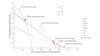
Figure 1: The Wage Frontier at a Four-Technique Patterns

1.0 Introduction

This post presents another numerical example of one technique replacing another, along the wage frontier, with a perturbation of a model parameter.

In a previous post, I identified three sequences of patterns of switch points in which the wage curves for one technique replaces the wage curve of another. In one of these sequences, a three-technique pattern removes the middle technique from three techniques with wage curves on the wage frontier. A further perturbation of the model parameter of concern results in another three technique pattern, in which the wage curve for a new technique appears in the middle of the wage frontier. In a limiting case of this sequence of patterns, the distance in the parameter space between the two three-technique patterns reduces to zero. A four-technique pattern results.

The parameter that is increased, in this case, is not a coefficient of production. Rather, I consider a model in which barriers to entry, or some such idiosyncratic property of investment in specific industries, results in maintaining specified ratios of the rates of profits among industries. One of these ratios is the parameter that is varied in the numerical example. I have applied my pattern analysis in a limited way to such a model before. By the way, although others have recently analyzed such a model, I find that Ian Steedman outlines this model in his 1977 book, Marx after Sraffa.

This example is more complicated than previous examples of four-technique patterns. At the switch point in which the wage curves for four techniques intersect, processes in two industries are both changed. This is a fluke case - a pattern of co-dimension two, in my terminology. But, in the example, the process in a third industry does not vary with the cost-minimizing techniques around the switch point. The example also illustrates variation in the sequence of switch points, at another region in the wage frontier, with the perturbation of a model parameter. I am not totally happy with this example. The wage curves are often curved more sharply than is seen in real-world data. If I am going to look at a three-commodity example, I would like to find one where at least two wage curves intersect three times for positive, feasible rates of profits.

When I applied the terminology of co-dimension to patterns, I expected that it would be difficult to find, through numerical experimentation, examples of patterns of higher co-dimension. I expected I would have to consciously try to create them, as I did for this example of a global pattern. I argued at one point that patterns of co-dimension one are important for seeing how the sequence of switch points along the wage frontier can change with technical progress or changes in the strength of barriers to entry and so on. I am now leaning towards thinking this argument applies to at least some patterns of higher co-dimension.

Anyways, this example illustrates complications that can arise in price theory that I do not think have been previously noted.

2.0 Technology

The technology in this example is almost the same as in one of my previous examples. I modified one labor coefficient. The economy produces a single consumption good, called corn. Corn is also a capital good, that is, a produced commodity used in the production of other commodities. In fact, iron, steel, and corn are capital goods in this example. So three industries exist. One produces iron, another produces steel, and the last produces corn. Two processes exist in each industry for producing the output of that industry. Each process exhibits Constant Returns to Scale (CRS) and is characterized by coefficients of production. Coefficients of production (Table 1) specify the physical quantities of inputs required to produce a unit output in the specified industry. All processes require a year to complete, and the inputs of iron, steel, and corn are all consumed over the year in providing their services so as to yield output at the end of the year.

Table 1: The Technology

Input	Iron Industry		Steel Industry		Corn Industry
	a	b	c	d	e	f
Labor	1/3	1/10	5/2	7/20	1	3/2
Iron	1/6	2/5	1/200	1/100	1	0
Steel	1/200	1/400	1/4	3/10	0	1/4
Corn	1/300	1/300	1/300	0	0	0

A technique consists of a process in each industry. Table 2 specifies the eight techniques that can be formed from the processes specified by the technology. If you work through this example, you will find that to produce a net output of one bushel corn, inputs of iron, steel, and corn all need to be produced to reproduce the capital goods used up in producing that bushel.

Table 2: Techniques

Technique	Processes
Alpha	a, c, e
Beta	a, c, f
Gamma	a, d, e
Delta	a, d, f
Epsilon	b, c, e
Zeta	b, c, f
Eta	b, d, e
Theta	b, d, f

Each technique is represented by coefficients of production. For the Alpha technique, let a_{0, α} be a three-element row vector representing the labor coefficients, and let A_α be the 3 x 3 Leontief matrix for this technique. The first element of a_{0, α}, (1/3) person-years per ton, represents the labor input needed to produce a ton of iron. The first column of A_α represents the inputs of iron, steel, and corn needed to produce a ton of iron. A parallel notation is used for the other seven techniques.

3.0 The Price System

Prices of production are defined to be constant spot prices that allow the smooth reproduction of the economy. Suppose Alpha is the cost-minimizing technique. Let p be the three-element row matrix designating the prices of iron, steel, and corn. I make the assumption that markets are such that the rate of profits in the iron, steel, and corn industries are (r s₁), (r s₂), and (r s₃), respectively. Suppose S is a diagonal matrix with the obvious elements along the diagonal, and I designates the identity matrix. Then prices of production satisfy the following system of equations:

p_α A_α (I + r S) + w_α a_{0, α} = p_α

I choose a bushel of corn to be the numeraire. If e₃ is the last column of the identity matrix, the following equation specifies the numeraire:

p_α e₃ = 1

As is not surprising, the above system of equations has one degree of freedom. One can solve for the wage, w_α(r), as a function of the scale factor for the rate of profits, r. The is a downward-sloping curve that intercepts both the axis for the wage and the scale factor at positive values. A similar function can be derived the other techniques, and they can be graphed in the same diagram.

4.0 The Choice of Technique

Figure 2 graphs the wage curves for all eight techniques, given specific values for the mark-ups, s_i, i = 1, 2, and 3. The outer envelope, called the wage frontier, represents the cost-minimizing technique for any given wage or scale factor for the rate of profits. (Although it is difficult to see in the graph, the Theta technique is cost-minimizing for a continuum of the wage between two switch points.) Notice that only two wage curves intersect at each switch point on the frontier. The techniques that are cost-minimizing at each switch point differ in only one process. This is a non-fluke example, for these markups. For what it is worth, the switch point between the Delta and Gamma techniques exhibits capital-reversing.

Figure 2: The Wage Frontier Before a Four-Technique Pattern

Table 3 shows the sequence of techniques that are cost-minimizing, along the wage frontier, at selected values of the markup for the iron industry. Figure 1, at the top of the post, illustrates the middle row. Presumably, two three-technique patterns have removed the Alpha and Gamma techniques from the frontier, for high values of the scale factor for the rate of profits. For the purposes of this post, I am not interested in those patterns. My point is focused on the switch point between the Eta and the Delta technique. Looking above at Table 2, one can see that, for these techniques, both processes in both the iron and corn industries are part of cost-minimizing techniques at the switch point. It follows that the Gamma and Theta techniques are cost-minimizing at this switch point, even though they do not appear on the wage frontier elsewhere. This is a fluke.

Table 3: Cost-Minimizing Techniques

s1	s2	s3	Techniques
3/2	1	1	Eta, Theta, Delta, Gamma, Alpha, Beta
2.665	1	1	Eta, Delta, Beta
4	1	1	Eta, Gamma, Delta, Beta

Finally, Figure 3 shows the wage frontier at the last level of the markup in the iron industry that I want to consider. The sequence of cost-minimizing techniques of Eta, Theta, and Delta, for relatively low scale factors for the rate of profits, has been replaced by the sequence of Eta, Gamma, and Delta. This example shows one sequence for how the wage frontier can be varied by lasting changes in a markup in one industry.

Figure 3: The Wage Frontier After a Four-Technique Pattern

5.0 Conclusion

Simple numerical examples are often presented in textbooks, such as Kurz and Salvadori's Theory of Production. They are often meant to illustrate phenomena that can appear in a more complicated example of a model. This post is an illustration of a fairly complicated example, where parts, in some sense, resemble simpler examples.