The question investigated here is whether Equation 9 is an implication of neoclassical microeconomics. I claim Equation 9 is not an implication of neoclassical microeconomics.
It is sufficient to demonstrate this negative conclusion by describing an example compatible with neoclassical microeconomics, but in which Equation 9 does not hold. The existence of such a counterexample demonstrates the use in macroeconomics of models in which the marginal product of capital and the interest rate are equal cannot claim full generality. It is up to the users of such models to state their assumptions and justify their use of these special cases.
How is the counter-example constructed? Assume we observe that in our economy only two goods are produced, steel and wheat, each measured in their own physical units, tons and bushels, respectively. We also observe the physical quantity flows in each industry, which I am going to write in a somewhat cryptic manner. Define d(0) as in Equation 12:
Suppose the physical quantity flows, on a per worker basis, are as Table 1. All quantities in the table are positive and:(12)
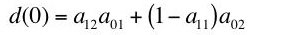
Notice that the sum of person-years across industries is unity, as promised. Also notice that the sum of the inputs of steel is equal to the steel produced by the steel industry. As a further clarification, we observe that these inputs are purchased at the beginning of the year, and the outputs become available at the end of the year. Furthermore, the steel input is totally used up in these production processes. The output of the steel industry just replaces the steel used up in the economy. The net output consists solely of wheat, which we observe to be a consumption good.(13)

| INPUTS HIRED AT START OF YEAR | STEEL INDUSTRY | WHEAT INDUSTRY | |
|---|---|---|---|
| Labor (Person-Years) |  | 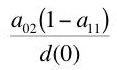 | |
| Steel (Tons Steel) |  | 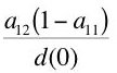 | |
| OUTPUTS |  |  |
Assume constant returns to scale. This means we can express the observed quantity flows as in Table 2. This explains the puzzling notation in Table 1. The parameters reflect unit (gross) outputs in both industries.
| INPUTS HIRED AT START OF YEAR | STEEL INDUSTRY | WHEAT INDUSTRY | |
|---|---|---|---|
| Labor |  Person-Years Person-Years |  Person-Years Person-Years | |
| Steel |  Tons Steel Tons Steel |  Tons Steel Tons Steel | |
| OUTPUTS | 1 Ton Steel | 1 Bushel Wheat |
Notice nothing has been assumed about the available technology other than constant returns to scale and that these proportions are possible. Based on our observations of the quantity flows actually used in this little model economy, we can draw no conclusions about what outputs will be produced when the inputs of either industry are in different proportions. It might even be the case that wheat can be used as a capital good for some other technology, or that copper or some other capital good might be used at a different set of prices.
We have observed that
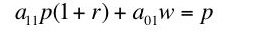
tons steel per worker are used in the economy, but this is not the value of capital per worker, k, used in Equation 5. The units are different. If aggregate output per head, y, is measured in units of bushels wheat per capita, capital per head, k, must also be measured in bushels wheat per capita in the aggregate production function framework. We have to figure out how many bushels of wheat this quantity of steel represents. But that's what prices are for.Suppose we observe that prices are unchanged over the year in which we are making our observations, and that the wage w is paid at the end of the year. Suppose that we also observe that competition has brought about the same rate of interest in both industries. Let wheat be numeraire. Then the following price equations obtain:
(14)
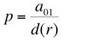
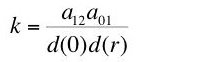
I have not specified enough equations to fully define the price system. Thus, we can solve for two of the price variables in terms of the third, say the rate of interest. Define d(r) as in Equation 16:(15)

The price of a ton of steel as a function of the interest rate is then given by Equation 17:(16)

Hence, the quantity of steel, when measured in bushels wheat, is:(17)
This value quantity of steel varies with the interest rate.(18)
The wage can also be found as a function of the rate of interest:
Equation 19 expresses the factor price curve [6] associated with the observed technique. A different technique, with its own factor price curve, may be preferred at a different rate of interest. All these curves can be graphed on the same diagram with the wage as the ordinate and the interest rate as the abscissa. The cost-minimizing technique(s) at any interest rate will correspond to the technique(s) with the highest wage at that interest rate [7]. The factor price frontier is thus formed from the outer-envelope curve of the factor price curves corresponding to each individual technique. Points on this frontier that lie on two or more curves for individual techniques are known as switch points. The optimal cost-minimizing technique is unique at interest rates for non-switching points.(19)

Assume the observed technique is a non-switching point. In the case of a discrete technology, the factor price curve for the selected technique is tangent to the factor price frontier at this rate of interest. The desired derivative, dw/dr, in Equation 9 is the slope of the factor price frontier at the observed rate of interest. From this tangency relationship one can see that the slope can be found by differentiating Equation 19, the factor price curve for the observed technique (Figure 2).
 |
| Figure 2: Factor-Price Curve For Cost-Minimizing Technique At Non-Switching Point |
Now we can return to our problem of examining Equation 9 for this simple two-good model. From Equation 19, the slope of the factor price frontier is given by Equation 20:
We can now compare the value of capital with the additive inverse of the tangent to the factor price frontier. The right hand sides of Equations 18 and 20 do not look like additive inverses of one another. As a matter of fact, assuming a positive interest rate, the interest rate is equal to the marginal product of capital at any given interest rate if Equation 21 holds:(20)

So if neoclassical theory is compatible with a steady state in which Equation 21 does not hold, macroeconomic models in which the interest rate is equated to the marginal product of capital are not the general case.(21)

Equation 21 is quite interesting. It implies that equilibrium prices are proportional to labor values, as defined in classical economics. As a matter of history, the reliance of the labor theory of value on this sort of extremely special case was thought to be a major weakness. If neoclassicals find this condition too extreme for the labor theory of value, they can hardly find it general enough as a defense of neoclassical macroeconomics [10].
Perhaps the solution lies in adopting another method of evaluating the physical quantity of capital in the same units as net output. Champernowne has proposed a chain index measure of capital that will restore the macroeconomic equality [11]. However, this measure only works under special cases, too. Burmeister has shown that the macroeconomic equality can be established with this chain-index if and only if real Wicksell effects are always negative. However, as was shown by the Cambridge Capital Controversy, this assumption of "negative real Wicksell effects" is not a general case either. In fact, nobody has determined what are necessary assumptions on technology to ensure the desired conclusion will follow [12]. Finally, if this index is used to express an aggregate production function in per capita terms, the wage is no longer equal to the marginal product of labor as that marginal product is typically expressed in such functions [13].
But, some may object, aggregate production functions work empirically. So even though economists cannot state their assumptions, they may say, this empirical success justifies the continual use of aggregate production functions. This is an extremely weak defense. Income distribution has been stable over much of the period in which macroeconomists have been using aggregate production functions. Franklin Fisher has shown through simulation that the supposed empirical success of aggregate production functions can arise under these conditions even in cases where the needed assumptions do not hold. Thus, this supposed empirical success of aggregate production functions fails to test the models with the unstated assumptions of aggregate neoclassical theory or to test among alternative theories. In fact, economists who rely on this defense seem to be confusing their empirical results with another accounting relationship [14].
Footnotes
[6] See:
- Heinz D. Kurz, "Factor Price Frontier," The New Palgrave.
- Heinz D. Kurz and Neri Salvadori (1995). Theory of Production: A Long Period Analysis, Cambridge University Press.
- Luigi Pasinetti (1969). "Switches of Technique and the 'Rate of Return' in Capital Theory," Economic Journal: 508-513.
- P. Garegnani (1970). "Heterogeneous capital, the Production Function and the Theory of Distribution," Review of Economic Studies, v 37, (June): 407-36.
- Frank Hahn (1982). "The neo-Ricardians," Cambridge Journal of Economics, V. 6: 353-374.
- Paul A. Samuelson (1962). "Parable and Realism in Capital Theory: The Surrogate Production Function," Review of Economic Studies: 193-206.
[12] See the reference in footnote 4.
[13] Salvatore Baldone (1984), "From Surrogate to Pseudo Production Functions," Cambridge Journal of Economics, V. 8: 271-288. Baldone also shows Burmeister's claims are problematic when used to compare quasi-stationary economies with a positive rate of growth, instead of just stationary economies.
[14] Anwar Shaikh (1990). "Humbug Production Function," The New Palgrave: Capital Theory, Macmillan.


No comments:
Post a Comment