Elsewhere

The Banach-Tarski Paradox

• The Hahn-Banach theorem is related to how mainstream economics model perfect competition. The video above is mind-bending math.
• The Mountain Goat blog.
• A profile of some economists at Berkeley, some of who I have read when they collaborated with Thomas Piketty or A. Dube. I have read deLong, as well, of course.
• If you cannot name 'capitalism', 'neoliberalism', or 'neoclassical economics', it is difficult to criticize them. Here is a popular account about right-wingers crying about researchers daring to use such terms.
• I conclude with a recent talk, below, by Yanis Varoufakis on the need for pluralism in economics. He argues, at least (I still have more to watch):
• Economic theory can be performative, counter-performative, or reflexive (without using those terms).
• Time, money, debt, and interest rates do not appear in the models in the textbook.
• Markets can exist without a society being capitalist.
• Once you have learned all these models that have nothing to say about capitalism, you might possibly say something intelligent.

Yanis Varoufakis: From an economics without capitalism to markets without capitalism.

The Production Function In A Discrete Technology

Figure 1: Isoquants For The Production Function

1.0 Introduction

I often assume a discrete technology in my demonstrations that what many mainstream economists teach is mostly incoherent balderdash. Some incompetents have told me that such well-established results "just show that the particular production functions that you have chosen don't work. This is not a generic result." So, for my amusement, I will go through a simple example here to explain how any continuously differentiable production function can be approximated arbitrarily closely by the production function for a discrete technology.

By the way as far as I know, capital-reversing is consistent with continuously differentiable production functions. Does the late Emmanuel Farhi's work on this theme make progress on Wolfgang Eichert's work? I sometimes worry that a serious exploration by a mainstream economist of the Cambridge capital controversy would lead to psychological depression.

2.0 The Model

I consider a single sector of an economy where, say, Q tons steel are manufactured from inputs of labor and iron. The managers of firm know of S processes for producing steel, where each process is characterized by an ordered pair of coefficients of production. That is, the technology for making steel, T, is defined as:

T = { (a₀(s), a(s)) | s = 1, 2, ..., S }

In the sth process, the services of at least a₀(s) person-years of labor and a(s) tons iron must be applied for every ton steel produced.

With only two inputs, I can assume that labor coefficients are ordered to be increasing:

0 < a₀(1) < a₀(2) < ... < a₀(S)

And that iron coefficients are decreasing:

a(1) > a(2) > ... > a(S) > 0

With this specification of technology, one can formulate a linear program (LP). Let L be the person-years of labor available to this firm, and let X be the tons of iron available. Define q₁, q₂, ..., q_S to be the tons steel produced with each of the S processes. Consider the following LP:

Given T, L, and X, choose q₁, q₂, ..., q_S

To maximize Q = q₁ + q₂ + ... + q_S such that

a₀(1) q₁ + a₀(2) q₂ + ... + a₀(S) q_S ≤ L

a(1) q₁ + a(2) q₂ + ... + a(S) q_S ≤ X

q₁ ≥ 0, q₂ ≥ 0, ..., q_S ≥ 0

Let the solution of this LP be:

Q = F(L, X)

Then F is the production function for steel production.

3.0 Selected Properties of a Production Function

A production function as defined above exhibits constant returns to scale (CRS). Figure 1, at the top of this post, displays isoquants for a particular technology with S equal to four. Any point in the interior of the line seqment between (a₀(1) Q, a(1) Q) and (a₀(2) Q, a(2) Q), for example, is a switch point. The extremes are non-switching points, where only one process in the technology is operated.

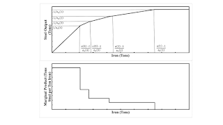
Figure 2 graphs the output of steel as a function of the labor input, given a specified quantity of iron available for input. The physical marginal product is shown below. The marginal product is non-increasing. The horizontal steps are non-switching points, and the vertical jumps occur at switch points.

Figure 2: The Marginal Product Of Labor

In this example, labor and iron inputs are treated formally the same. So, as Figure 3 shows, the graph of the output of steel as a function of the iron input, and of iron's physical marginal product, look qualitatively the same as the output of steel as a function of the labor input.

Figure 3: The Marginal Product Of Iron

Linear programming, as I understand it, is not taught as introductory mathematics. On the other hand, one can explain the above graphs without knowledge of calculus. Are there still recent introductory textbooks for microeconomics with graphs like the above?

4.0 Conclusions

One can generalize the above to consider a production function for more than two inputs. The processes will not be ordered as above, and isoquants would be graphed in a higher dimensional space. Another generalization would consider multiple production funtions, one for each sector, with given prices for the produced outputs. Given endowments for inputs, also known as 'factors of production', the dual problem assigns shadow prices to the inputs. Also, endowments are not given in long-period models.

References

• Eichert, Wolfgang. 2014a. Long-period positions in multi-sectoral Cobb-Douglas economies. Metroeconomica 65 (1): 136-153.
• Eichert, Wolfgang. 2014b. Technological Change in Multi-Sectoral Economies: Theoretical Change in Multi-Sectoral Economies. Doctoral thesis, University of Graz.
• Pasinetti, Luigi L. 1977. Lectures on the Theory of Production. New York: Columbia University Press.

Private Truths, Public Lies In Mainstream Economics?

I sometimes wonder if most mainstream economists think that most of what they were taught, teach, and research are some combination of false, incoherent, and useless for understanding actually existing capitalism. But they go along out of some sense of professionalism and a belief that their colleagues do not share their views. That is many privately think they are a minority of one, but publically espouse the orthodoxy.

As far as professionalism goes, I suppose some believe that those who go on from their microeconomics class, for example, are expected to have been exposed to certain material. I would hope that some question the ethics of not letting the students know that they are being taught one approach, named marginalism, and other approaches exist.

Maybe one of these days, I will read Timur Kuran's book.

Bushwa From Jeffrey Clemens In The Journal of Economic Perspectives

"The labor supply curve slopes upward, reflecting differences in workers’ reservation wages (as driven by outside opportunities related, perhaps, to leisure, home production, and economic assistance that can be received while out of work). The labor demand curve slopes downward, tracing out the relationship between the quantity of labor employed and the marginal revenue product of that labor. This, in turn, reflects the assumption of a constant price (due, perhaps, to a perfectly competitive market for the firm’s output) and a production function in which, holding capital and technology fixed, labor has diminishing marginal productivity.

In a perfectly competitive labor market, a freely set wage will adjust to equilibrate supply and demand..."

-- Jeffrey Clemens. 2021. How do firms respond to minimum wage increases? Understanding the relevance of non-employment margins. Journal of Economic Perspectives (Winter): 51 - 72.

Clemens then considers shifts in demand and supply curves for labor with changes in prices due to market power in final goods, changes in benefits, and other aspects of jobs. He never notes his framework is balderdash. Empirical evidence, which Clemens cites, cannot make up for his basic incoherence. Mayhaps, Clemens could read Fabio Petri's textbook when it is published.

I do not expect to read articles about the speed of the ether in absolute space in physics journals. Nor do I expect to read about the weight of phlogiston in chemistry journals. Why does the American Economic Association publish articles that make astrologists look good?