Absolute Rent, Extensive Rent, And Intensive Rent

Figure 1: Rent Curves With and Without Competitive Markets

This post is a continuation of the example in this and this post. It is the first example, in the tradition building on Sraffa, of a numerical example combines absolute, intensive, and extensive rent.

The analysis in those posts can be extended to apply to non-competitive markets. Assume that the rate of profits is s₁ r in the price equation for the process producing iron and s₂ r in any process for producing corn. I now call r the scale factor for the rate of profits. As a normalization, let the sum of s₁ and s₂ be unity. These coefficients are given parameters. They express the existence of persistent barriers to entry between industry and agriculture. For concreteness, I take s₁ ≈ 0.0208506. This parameter expresses a case of the reswitching of the order of rentability, with agriculture obtaining a higher rate of profits than industry.

Capitalists in agriculture have market power in this post. The changes in rent, including increases, is not the result of market power by landlords. The increased market power of farmers changes wage and rent curves. The specific parameters for markups considered here eliminate the reswitching of techniques and capital-reversing, at any level of net output. Otherwise, the capital-intensity of industries is not analyzed in this post. For Marx, absolute rent is created from more surplus value being generated in agriculture, given its low organic composition of capital. This additional surplus value is not shared in a common pool because of the market power of the class of landlords. This article neither investigates nor justifies Marx's specific mechanism. Nevertheless, I identify the differences in rent brought about relative market power among capitalists in different economic sectors with absolute rent.

The price systems for each technique are altered by the differences in relative markups between industry and agriculture. The variation of the feasibility of techniques with net output is independent of prices. Table 3, in this post, applies to this numerical example of a model of non-competitive markets. Omicron, Rho, Tau, and Omega remain feasible at the highest level of net output. Figure 2 presents the wage curves for this example of non-competitive markets, and Figure 3 is a detail.

Figure 2: Wage Curves With Non-Competitive Markets

Figure 3: Wage Curves With Non-Competitive Markets (Detail)

With these specific values for relative markups, Omicron and Rho are each cost-minimizing for a range of the scale factor for the rate of profits when net output is towards its maximum (Table 5). Type 1 land is not scarce and pays no rent when Omicron is cost-minimizing. Type 2 land is not scarce under Rho. At the highest level of net output, only extensive rent is obtained. No intensive rent is paid, whatever value the scale factor for the rate of profits takes on. The orders of efficiency and rentability match and do not vary with the scale factor for the rate of profits when Omicron is cost-minimizing. The order of efficiency varies, when Rho is cost-minimizing. Rho exhibits the reswitching of the order of rentability.

Table 1: Cost-Minimizing Technique

Range	Technique	Order of Efficiency	Order of Rentability
0≤r≤9.5%	Omicron	3,2,1	3,2,1
9.5≤r≤41.7%	Rho	3,1,2	3,1,2
41.7≤r≤87.8%		1,3,2
87.8≤r≤114.9%			1,3,2
114.9≤r≤122.0%			3,1,2

Figure 1, at the top of this post, graphs the rent curves for the example. Both the wage and rent per acre are functions of the (scale factor for the) rate of profits. The analysis of the choice of technique would be different if the wage were taken as given exogenously. In the case in this post, rent per acre is less under Omicron when the capitalists in agriculture have more market power. The variation in rent per acre with increased market power for farmers otherwise reflects the change in the cost-minimizing technique. Landlords who own Type 1 land obtain greater rent from the increased market power for agriculture in the example. The same is true for landlords who own Type 3 land, expect for low rates of profits. Landlords who own Type 2 land, on the other hand, are better off with competitive markets.

This level of increased market power for the capitalists in agriculture alters the analysis the choice of technique at every level of net output (Figure 4). Consider the range of the scale factor for the rate of profits at which Delta is cost-minimizing. As output expands, at the bottom of this range, capitalists choose to operate processes IV and V on Type 3 land to expand output. When output can no longer be expanded by extending cultivation with process IV, they bring Type 2 land under cultivation, and then, with the adoption of Omicron, Type 1 land enters into the mix. At a slightly higher scale factor, the capitalists cultivate Type 1 land after Type 3 land is completely farmed with process IV. Ultimately, under Rho, they also cultivate Type 2 land. Consider a still higher scale factor, but still within the range where Delta is initially cost-minimizing. The capitalists first expand output, when Type 3 land is fully cultivated, by starting to farm Type 1 land. They operate processes IV and V side-by-side on Type 3 land only after Type 1 land has become scarce.

Figure 4: Cost-Minimizing Techniques With Non-Competitive Markets

In all of these cases, and for even a higher scale factor, process IV is ultimately operated on Type 3 land alone, and only extensive rent is obtained. Yet, with intensive rent being obtained somewhere along the expansion of output, process V enters into the determination of the order of efficiency. The switch points between the wage curves for Alpha and Gamma and between Alpha and Phi are irrelevant to the determination of the order of efficiency when Rho is cost-minimizing. The order of efficiency varies, though, around the switch point between Alpha and Delta. As with competitive markets, the existence of intensive rent as output expands affects the order of efficiency under extensive rent at the highest level of output.

Problems With The Economic Calculation Problem

Hakim on the Economic Calculation Problem

Reactionaries often bring up the Economic Calculation Problem (ECP) as a fatal objection to socialism, considered as entailing central planning. Ludwig Von Mises put this forth in 1920 as an argument in principle that central planning is guaranteed to be highly inefficient. He postulates that the planning authority knows the prices of consumer goods and all technical possibilities, including the endowments of originary factors of production. But without prices of intermediate goods, the planning authority cannot make rational decisions about how to produce commodities. Like Enrico Barone, Von Mises insists the planning authority must re-introduce prices for intermediate goods and a market for 'capital'.

Friedrich Hayek changed the question. He argued that efficient central planning was impractical, not impossible in principle. For Hayek, prices bring about a coordination among entrepreneurs of their plans and expectations. Hayek raised the question on how the planning authority could gather the data they need for their equations. He emphasized dispersed tacit knowledge of time and space.

I emphasize that what the ECP is is disputable. Also, it is inapplicable to the ideas of anarcho-syndicalism, council communists, and so on. Anyways, this post poses some problems with using the ECP as an objection to socialist central planning.

Magnitude of costs of failures of coordination. Neither Von Mises nor Hayek attempt to estimate the costs of a failure of coordination. Since they say a capitalist economy will always be in a disequilibrium state, capitalism will also suffer costs of discoordination at any point of time. How much more are the costs in a centrally planned society, as opposed to a capitalist society? What is the empirical evidence that the ECP was a major problem for the U.S.S.R?

Externalities. For economists of the Austrian school, the extent of the coordination of plans and expectations of diverse agents is a criterion for welfare economics. This approach contrasts with the maintream marginalist criteria of Pareto and Hicks-Kaldor efficiency. The approach of the Austrian school does not seem to me to adequately account for externalities, such as global warming. To Von Mises' credit, he does bring up the destruction of the unpriced natural beauty of a waterfall in discussing its use for power generation.

How do prices bring about coordination? To me, when Hayek describes economic coordination, he is describing something like Hicks' model of temporary equibrium, as in Value and Capital, or the Arrow-Debreu model of intertemporal equilibria, as in Debreu's Theory of Value. Much research suggests such a coordinated state cannt be expected to be brought about by disequilibrium market processes. (Issues exist in how my favorite model can describe trends in capitalist economies, particularly in accounting for if joint production.)

Mises is mathematically mistaken. Suppose prices of commodities provided as components of final demand, technical possibilies, and endowments of originary factors of production are given to the Ministry of Planning. The level at which to operate each production process is found as the result of the solution to an optimization problem. One does not need prices of factors of production to solve the primal problem. Such prices emerge as the solution of the dual problem. Von Mises' mistakes and dogmatism may have been useful in that they encouraged others to explore one approach to price theory.

Mises and Hayek misunderstand capitalism. Anyways, most prices in a capitalist economy do not communicate knowledge like Hayek describes. They do not continuously fluctuate under the influence of supply and demand. Rather, prices of manufactured commodities are usually full cost prices or administrated prices, set by firms. Variations in the level of output, inventories, and queues of orders are of some importance.

Above, I have not said anything about improvements in computer networks or computer speed. I do not see how IBM'a North Pole computer (Modha's blog) would be helpful in linear programming. Hakim recomments Cottrell and Cockshott (1993) for those who want to know more about the ECP. I have not read The People's Republic of Walmart, which some recommend.

How To Find Fluke Switch Points

Figure 1: Convergence of Newton Method

This post steps through an algorithm for finding a fluke switch point. I used a different example when I tried to explain this before. Today, I use an example building on my draft ROPE Article.

Consider Figure 3 in this post, repeated below as Figure 2. Let s₁ = s₂ = 1. I want to find s₃, the markup in the corn industry, such that the wage curves for Gamma, Delta, Eta, and Theta intersect at a single switch point. One wants to find a function one of whose zeros is the desired markup.

Figure 2: Variation of Switch Points with the Markup in the Corn Industry

This economy produces a single consumption good, called corn. Corn is also a capital good, that is, a produced commodity used in the production of other commodities. In fact, iron, steel, and corn are capital goods in this example. So three industries exist. One produces iron, another produces steel, and the last produces corn. Two processes exist in each industry for producing the output of that industry. Each process exhibits Constant Returns to Scale (CRS) and is characterized by coefficients of production. Coefficients of production (Table 1) specify the physical quantities of inputs required to produce a unit output in the specified industry. All processes require a year to complete, and the inputs of iron, steel, and corn are all consumed over the year in providing their services so as to yield output at the end of the year.

Table 1: The Technology

Input	Iron Industry		Steel Industry		Corn Industry
	a	b	c	d	e	f
Labor	1/3	1/10	5/2	7/20	1	3/2
Iron	1/6	2/5	1/200	1/100	1	0
Steel	1/200	1/400	1/4	3/10	0	1/4
Corn	1/300	1/300	1/300	0	0	0

A technique consists of a process in each industry. Table 2 specifies the eight techniques that can be formed from the processes specified by the technology. If you work through this example, you will find that to produce a net output of one bushel corn, inputs of iron, steel, and corn all need to be produced to reproduce the capital goods used up in producing that bushel.

Table 2: Techniques

Technique	Processes
Alpha	a, c, e
Beta	a, c, f
Gamma	a, d, e
Delta	a, d, f
Epsilon	b, c, e
Zeta	b, c, f
Eta	b, d, e
Theta	b, d, f

Given the markups s₁, s₂, and s₃, the wage and prices under Gamma are rational functions of the scale factor for the rate of profits:

w_γ(r) = (f₃ r³ + f₂ r² + f₁ r + f₀)/(g₂ r² + g₁ r + g₀)

p_γ,1(r) = (u₂ r² + u₁ r + u₀)/(g₂ r² + g₁ r + g₀)

p_γ,2(r) = (v₂ r² + v₁ r + v₀)/(g₂ r² + g₁ r + g₀)

Since corn is the numeraire, its price is unity. The coefficients of the polynomials are functions of the coefficients of production for the first, second, and first processes in the iron, steel, and corn industries, respectively, and of the markups.

The Delta technique differs from Gamma in the process for producing corn. The extra profits obtained in operating the second corn-producing process at Gamma prices are:

h₁(r)/(g₂ r² + g₁ r + g₀) = 1

- [(a_f,1,3 p_γ,1(r) + a_f,2,3 p_γ,2(r) + a_f,3,3)(1 + s₃r)

+ a_f,0,3 w_γ(r)]

A switch point between Gamma and Delta is found as an appropriate zero of h₁(r), which is a cubic polynomial. Denote r₁(s₃) as the zero sought for the fluke case.

The extra profits obtained in operating the second iron-producing process at Gamma prices are:

h₂(r)/(g₂ r² + g₁ r + g₀) = p_γ,1(r)

- [(a_b,1,1 p_γ,1(r) + a_b,2,1 p_γ,2(r) + a_b,3,1)(1 + s₁r)

+ a_b,0,1 w_γ(r)]

An appropriate zero of h₂(r) is a switch point between Gamma and Eta. Denote r₂(s₃) as the zero sought for the fluke case.

Consider the following function:

h(s₃) = r₂(s₃) - r₁(s₃)

A zero of h(s₃) is such that the wage curves for Gamma, Delta, Eta, and Theta intersect at a single switch point. At a switch point for Gamma, Delta, and Eta, neither extra profits nor extra costs will be obtained in operating either iron-producing and corn-producing processes. Since the same steel-producing process is operated in all four techniques, Theta is also cost-minimizing at this switch point.

One can find such a zero by applying Newton’s method to two initial guesses, as illustrated in Figure 1 at the top of the post. Some experimentation allows one to determine two initial guesses, s⁰₃ and s¹₃, for the markup in the corn industry and for which roots of the cubics are wanted. The slope of a linear approximation to the function whose zero is sought is:

m_{i + 2} = [h(sⁱ₃) - h(s^{i + 1}₃)]/(sⁱ₃ - s^{i + 1}₃), i = 0, 1, 2, ...

The intercept with the ordinate is:

b_{i + 2} = h(s^{i + 1}₃ - m_{i + 2} s^{i + 1}₃, i = 0, 1, 2, ...

The next iteration is:

s^{i + 2}₃ = - b_{i + 2}/m_{i + 2}, i = 0, 1, 2, ...

In my experience, Newton's method converges fairly rapidly in this application of finding fluke switch points.

Variation With Markups Of The Analysis Of The Choice Of Technique With Intensive Rent

Figure 1: Variation of the Technique with Markup in Agriculture

This post is a continuation a of a previous example.

I suppose this is the first example in post Sraffian price theory which combines intensive rent and markup pricing. I do not plan on trying to publish it, in a stand-alone article. D'Agata (1983) sets some coefficients to zero to simplify it for his purposes. I would like a range of parameters where I get reswitching or capital-reversing. I have found a case where, given the wage, the cost-minimizing technique is not unique away from switch points. I would like an example where some of the locii in Figure 2 below intersect.

I might as well repeat the data. Table 1 shows the coefficients of production. Only one type of land exists, and three processes are known for producing corn on it. Following D'Agata, assume that one hundred acres of land are available and that net output consists of 90 tons iron, 60 tons steel, and 19 bushels corn. The net output is also the numeraire.

Table 1: The Coefficients of Production

Input	Industry
	Iron	Steel	Corn
	I	II	III	IV	V
Labor	1	1	1	11/5	1
Land	0	0	1	1	1
Iron	0	0	1/10	1/10	1/10
Steel	0	0	2/5	1/10	1/10
Corn	1/10	3/5	1/10	3/10	2/5

All three commodities must be produced for any composition of net output. Table 2 lists the available techniques. Only Alpha, Delta, and Epsilon are feasible for these requirements for use. Not all land is farmed and only one corn-producing process is operated under Alpha. Two corn-producing processes are operated together under Delta and Epsilon.

Table 2: Techniques

Technique	Processes
Alpha	I, II, III
Beta	I, II, IV
Gamma	I, II, V
Delta	I, II, III, IV
Epsilon	I, II, III, V
Zeta	I, II, IV, V

In the non-competitive case, the relative markups in different industries are taken as given. Let the rates of profits be in proportions of s₁, s₂, and s₃, respectively.

Figure 1, at the top of the post, shows the variation in the analysis of the cost-minimizing technique with perturbations of the markup up in agriculture. In drawing this figure, markups in iron and corn production, s₁ and s₂, are assumed unity. At the intersection between the Alpha and Delta wage curves, the rent for Delta is zero. The scale factor at this switch point is the maximum for the Delta technique. At a switch point between Alpha and Epsilon in regions 1, 2, 3, and 4, the rent for epsilon is zero. The scale factor at such a switch point is the maximum scale factor for Epsilon. In regions 5 and 6, the maximum scale factor for Epsilon is the scale factor for which the wage turns negative.

A fluke case exists off to the right where the wage curves for Alpha at Delta intersect at the maximum scale factor for the rate of profits for Alpha. At that switch point, Delta has a scale factor for the rate of profits of zero percent and a rent of zero. The fluke case partitioning regions 2 and 3 is one where the wage curves for Alpha and Epsilon intersect at the scale factor where the wage for Delta first turns positive. The fluke case partitioning regions 3 and 4 is one in which the wage curves for Alpha, Delta, and Epsilon all intersect at a single switch point.

The fluke cases partition regions 4 & 5 and 5 & 6 change some characteristics of the range of the scale factor of the rate of profits in which no cost-minimizing technique exists. At the fluke case partitioning regions 4 and 5, the wage curves for Alpha and Epsilon intersect at the maximum scale factor for Alpha. I have previously provided an analysis of the fluke case dividing regions 5 and 6. Maybe I should not consider these two fluke cases since they arise, in some sense, for switch points off the frontier.

Anyways, Table 2 shows how the analysis of the choice of technique varies among the numbered regions. If wants to look at these results in some detail, one can relate the variation in the analysis of the choice of technique to the fluke cases.

Table 2: The Cost-Minimizing Technique in Selected Regions in Parameter Space

Region	Range for Scale Factor	Cost-Minimizing Techniques
1	0 ≤ r ≤ R*,ε	Epsilon
	R*,ε ≤ r ≤ Rα	Alpha
2	0 ≤ r ≤ R*,ε	Epsilon
	R*,ε ≤ r ≤ Rδ	Alpha
	Rδ ≤ r ≤ R*,δ	Alpha and Delta
	R*,δ ≤ r < Rα	None. Wage for Alpha positive.
3	0 ≤ r ≤ Rδ	Epsilon
	Rδ ≤ r ≤ R*,ε	Delta and Epsilon
	R*,ε ≤ r ≤ R*,δ	Alpha and Delta
	R*,δ ≤ r < Rα	None. Wage for Alpha positive.
4	0 ≤ r ≤ Rδ	Epsilon
	Rδ ≤ r ≤ r*	Delta and Epsilon
	r* ≤ r ≤ R*,δ	None. Wage for Alpha, Delta, Epsilon positive. Rent for Delta and Epsilon positive.
	R*,δ ≤ r < R*,ε	None. Wage for Alpha and Epsilon positive. Rent for Epsilon positive.
	R*,ε ≤ r < Rα	None. Wage for Alpha positive.
5	0 ≤ r ≤ Rδ	Epsilon
	Rδ ≤ r ≤ r*	Delta and Epsilon
	r* ≤ r ≤ R*,δ	None. Wage for Alpha, Delta, Epsilon positive. Rent for Delta and Epsilon positive.
	R*,δ ≤ r ≤ Rε	None. Wage for Alpha, Epsilon positive. Rent for Epsilon positive.
	Rε ≤ r < Rα	None. Wage for Alpha positive.
6	0 ≤ r ≤ Rδ	Epsilon
	Rδ ≤ r ≤ r*	Delta and Epsilon
	r* ≤ r ≤ Rε	None. Wage for Alpha, Delta, Epsilon positive. Rent for Delta and Epsilon positive.
	Rε ≤ r ≤ R*,δ	None. Wage for Alpha, Delta, positive. Rent for Delta positive.
	R*,δ ≤ r < Rα	None. Wage for Alpha positive.

Figure 2, for completeness, illustrates the partition of the parameter space of markups, where the ratios of markups in iron and steel need not be the same. Figure 1 illustrates what happens along a vertical line in Figure 2 at s₂/s₁ is unity. I realize it is hard to see region 4 and to distinguish its boundaries in Figure 2.

Figure 2: Partition Of Parameter Space

I do not draw any great conclusions. This example demonstrates my visualization techniques and perturbation analysis can be applied to an example where the cost-mninimizing technique is not found from a frontier of wage curves. The non-uniqueness and non-existence of a cost-minimizing technique arises in D'Agata's original example.

An Alpha Vs. Delta Pattern For The r-Order Of Fertility With Intensive Rent And Markup Pricing

Figure 1: Wage Curves and Rent for an Example of Intensive Rent

This post is a continuation of a previous example.

This is a fluke case insofar as the Alpha and Delta wage curves intersect at the scale factor for the rate of profits that is the maximum possible for the Epsilon technique. This fluke case is associated with a qualitative change in the range of the scale factor for the rate of profits in which no cost-minimizing technique exists.

The technology, endowments, requirements for use, and techniques are as previously defined. Requirements for use can only be satisfied by the Alpha, Delta, and Epsilon techniques.

I continue to consider markup pricing. The rate of profits is (s₁ r), (s₂ r), and (s₃ r) in the iron, steel, and corn industries. In determining which technique is cost-minimizing, r, the scale factor for the rate of profits is taken as given.

Figure 1, at the top of this post, depicts the wage and rent curves for the different techniques. The wage curves for the cost-minimizing techniques lie on the wage frontier. The wage frontier consists of the wage curves for the Delta and Epsilon techniques up to the switch point between them. The wage frontier ends there. No technique is cost-minimizing between this switch point and the maximum scale factor for the rate of profits for Alpha.

Table 1 goes into more detail on the wage curves than aqnybody probably cares about. I introduce some notation that I will find useful in later posts. R_δ is the scale factor for the rate of profits at which the wage is zero for Delta. R_*,δ is the scale factor for the rate of profits at which the rent is zero for Delta. This is a fluke case because R_*,δ is equal to R_ε. Anyways, in the first range for the scale factor, only the Alpha and Epsilon techniques have wage curves that are eligible to lie on the wage frontier; the wage curve for the Delta technique lies below the axis for the scale factor for the rate of profits. In the next two ranges, all three wage curves are eligible. In the last range of the scale factor, only the wage curve for Alpha is eligible. The rent curve for Delta and the wage curve for Epsilon lie below the axis for the scale factor.

Table 1: Cost-Minimizing Techniques

Lower Bound on r	Upper Bound on r	Techniques
0 percent	Rδ	Alpha has a positive wage
		Delta has a negative wage
		Epsilon has a positive wage and positive rent
		Epsilon is uniquely cost-minimizing
Rδ	r*	Alpha has a positive wage
		Delta has a positive wage and positive rent
		Epsilon has a positive wage and positive rent
		Delta is non-uniquely cost-minimizing
		Epsilon is non-uniquely cost-minimizing
r*	R*,δ	Alpha has a positive wage
		Delta has a positive wage and positive rent
		Epsilon has a positive wage and positive rent
		No cost-minimizing technique exists
R*,δ	Rα	Alpha has a positive wage
		Delta has a positive wage and negative rent
		Epsilon has a negative wage and positive rent
		No cost-minimizing technique exists

I plot extra profits for each process for each technique to demonstrate my claims about which technique is cost-minimizing. Figure 2 shows extra profits for each process at Alpha prices. Extra profits are zero for the three processes comprising the technique. The last corn-producing process can always pay extra profits for any scale factor, while the penultimate process can pay extra profits for any scale factor greater than that at the intersection of the Alpha and Delta wage curves and not exceeding the maximum scale factor for the Alpha technique. The Alpha technique is never cost-minimizing.

Figure 2: Extra Profits with Alpha Prices

Figure 3 plots extra profits for each process for the Delta and Epsilon techniques. Since four of the five processes in the technology are operated for each technique, four of the five processes obtain extra profits of zero for all scale factors between the limits for each technique. If the Delta technique were in operation at a scale factor greater than at the switch point between Delta and Epsilon, farmers would start to operate the fifth process, moving away from the Delta technique. If the Epsilon technique were in operation in this range, farmers would start to operate the fourth technique. A market algorithm would not coverge to any technique for a scale factor for the rate of profits greater than that at the switch point between Delta and Epsilon and not exceeding the maximum scale factor for the Alpha technique.

Figure 3: Extra Profits with Delta or Epsilon Prices

For a smaller markup in agriculture than in this fluke case, three interesting ranges of the scale factor exist where no technique is cost-minimizing. In the first, the Alpha, Delta, and Epsilon techniques can all pay positive wages and non-negative rents, with positive prices. In the second, only the Alpha and Delta techniques can pay positive wages and a non-negative rent. In the third, the Alpha technique can pay a positive wage, while the Delta technique cannot pay a positive rent.

For a larger markup than in the fluke case, the second interesting range of the scale factor has changed. The Delta technique can no longer pay a positive rent. Instead, the Alpha and Epsilon techniques can pay positive wages and non-negative rents, with positive prices.

A Pattern For The r-Order Of Fertility With Intensive Rent And Markup Pricing

Figure 1: Wage Curves and Rent for an Example of Intensive Rent

The first man who, having enclosed a piece of ground, bethought himself of saying, 'This is mine', and found people simple enough to believe him, was the real founder of civil society. From how many crimes, wars and murders, from how many horrors and misfortunes, might not anyone have saved mankind by pulling up the stakes, filling in the ditch, and crying to his fellows, 'Beware of listening to this imposter; you are undone if you once forget that the fruits of the earth belong to us all, and the earth itself to nobody.' -- Jean Jacques Rousseau

1.0 Introduction

This post is a continuation of a previous example. Three commodities, iron, steel, and corn, are produced commodities. A single type of land exists, and three processes are available for producing corn on land.

The choice of technique corresponds to the selection of which processes are used in agriculture. Only the Alpha, Delta, and Epsilon techniques are feasibles for the given endowment of land and the requirements for use. Under Alpha, the land is only partially farmed. Land is not scarce and obtains no rent. Under Delta and Epsilon, the land is fully farmed, with two corn-producing processes being operated side-by-side. The second of these processes varies between Delta and Epsilon.

2.0 Choice of Technique

Prices of production are assumed to prevail, but markups over costs vary between industry and agriculture.

Figure 1 illustrates the wage and rent curves for this example. For a non-negative scale factor for the rate of profits up to the first switch point point, the Epsilon technique is cost-minimizing. At this switch point, the rent on land for Epsilon is zero, while it is positive for any smaller non-negative scale factor. This switch point is a fluke in that it is also the scale factor for the rate of profits at which the wage first turns positive for the Delta technique.

Between this first switch point and the switch point between Alpha and Delta, both the Alpha and Delta techniques are cost-minimizing. At the second switch point, the rent on land for Delta is zero. For a scale factor somewhat larger than at this switch point, no technique is cost-minimizing. Delta and Epsilon are feasible, but rent is negative for both of them. The wage for Epsilon is also negative. Alpha, on the other hand, is feasible, can pay a positive wage, and has a non-negative (zero) rent. Prices of iron, steel, and corn for Alpha are also positive in this range. Yet Alpha is not cost-minimizing.

Table 1: Cost-Minimizing Techniques

Lower Bound on r	Upper Bound on r	Techniques
0 percent	r*	Alpha has a positive wage
		Delta has a negative wage
		Epsilon has a positive wage and positive rent
		Epsilon is uniquely cost-minimizing
r*	r**	Alpha has a positive wage
		Delta has a positive wage and positive rent
		Epsilon has a positive wage and negative rent
		Alpha is non-uniquely cost-minimizing
		Delta is non-uniquely cost-minimizing
r**	rα, max	Alpha has a positive wage
		Delta has negative rent
		Epsilon has negative wage and negative rent
		No cost-minimizing technique exists

Table 1 summarizes these claims about which techniques are cost-minimizing for which ranges of the scale factor for the rate of profits. Figure 2 graphs extra profits for each process at Alpha prices. Extra profits are the difference bewteen the price of the commodity produced by the process and the costs for commodity inputs, rent, and wages. The costs of inputs of iron, steel, and corn incur the going rate of profits for that industry, including markups. Extra profits can be positive or negative. As a check on the calculations, one can maybe see from the graph that extra profits are zero, neither positive nor negative, for the three processes comprising the Alpha technique. For a non-negative scale factor less than at the first switch point, extra profits can be made at Alpha prices by growing corn with the fifth process in the technology. For a scale factor exceeding that at the second switch point, but below the maximum, extra profits are obtained by growing corn with the fourth process in the technology. Thus, Alpha is only cost-minimizing between the switch points.

Figure 2: Extra Profits with Alpha Prices

Figure 3 shows the extra profits obtained for each process for the Delta and Epsilon techniques, in the left and right panes respectively. Extra profits are only graphed for each for the range of the scale factor for the rate of profits for which both the wage and rent is non-negative. Since four of the five processes are operated in Delta, or in Epsilon, extra profits are non-zero for only one process in each graph. And you can see both techniques are cost-minimizing for the full range of the graphed scale factor in each case.

Figure 3: Extra Profits with Delta or Epsilon Prices

3.0 Conclusion

For a markup in agriculture slightly lower than for the fluke case, a range of the scale factor for the rate of profits exists in which the Delta and Epsilon techniques are both cost-minimizing. For a markup slightly higher, no such range, not even a single point, exists. For the whole range of the scale factor in which the Delta technique exhibits a positive rate of profits and a positive rent, the Alpha technique is also cost-minimizing. And when the Alpha technique is cost-minimizing, the class of landlords cannot exist.

A Three-Technique Pattern With Intensive Rent And Markup Pricing

Figure 1: Wage Curves and Rent for an Example of Intensive Rent

1.0 Introduction

This post is one in a series exploring variations of an example from Antonio D'Agata (1983).

This post demonstrates that at least one of my fluke cases can appear in a model of intensive rent by varying a parameter specifying relative markups among sectors. This post is only a start of exploring the parameter space of relative markups in a specific numeric example of intensive rent.

Suppose the rate of profits is given, subject to the constraint that the ratios of the rate of profits in agriculture to that in other industries are as specified. Then the wage can be one of two distinct levels. When the wage is at the lower level, then the rent per acre is higher and vice versa. On the other hand, an increased wage, when it is at the lower level is associated with an increased rate of profits.

2.0 Technology, Requirements for Use, Endowments, and Relative Markups

Table 1 presents coefficients of production in an example from D'Agata (1983). Only one type of land exists, and three processes are known for producing corn on it. The scarcity of land is shown by the possibility of two corn-producing processes being operated side-by-side in the cost-minimizing technique.

Table 1: The Coefficients of Production

Input	Industry
	Iron	Steel	Corn
	I	II	III	IV	V
Labor	1	1	1	11/5	1
Land	0	0	1	1	1
Iron	0	0	1/10	1/10	1/10
Steel	0	0	2/5	1/10	1/10
Corn	1/10	3/5	1/10	3/10	2/5

Following D'Agata, assume that one hundred acres of land are available and that net output consists of 90 tons iron, 60 tons steel, and 19 bushels corn. The net output is also the numeraire. All three commodities must be produced for any composition of net output. Table 2 lists the available techniques. Only Alpha, Delta, and Epsilon are feasible for these requirements for use. Not all land is farmed and only one corn-producing process is operated under Alpha. Two corn-producing processes are operated together under Delta and Epsilon.

Table 2: Techniques

Technique	Processes
Alpha	I, II, III
Beta	I, II, IV
Gamma	I, II, V
Delta	I, II, III, IV
Epsilon	I, II, III, V
Zeta	I, II, IV, V

In the non-competitive case, the relative markups in different industries are taken as given. Let the rates of profits be in proportions of s₁, s₂, and s₃, respectively.

3.0 Prices of Production

Prices of prodution can be defined for each technique. Each process operated in a technique contributes an equation in which the going rate of profits are obtained for that industry. The rate of profits in producing iron is s₁ r. In steel, it is s₂ r, and it is s₃ r in the corn-producing processes. As in past posts, I call r the scale factor for the rate of profits.

For example, the following equations specify prices of production for the Delta technique:

(p₁ a_1,1 + p₂ a_2,1 + p₃ a_3,1)(1 + s₁ r) + w a_0,1 = p₁

(p₁ a_1,2 + p₂ a_2,2 + p₃ a_3,2)(1 + s₂ r) + w a_0,2 = p₂

(p₁ a_1,3 + p₂ a_2,3 + p₃ a_3,3)(1 + s₃ r) + ρ c₃ + w a_0,2 = p₃

(p₁ a_1,4 + p₂ a_2,4 + p₃ a_3,4)(1 + s₃ r) + ρ c₄ + w a_0,3 = p₃

In these equations, p₁, p₂, and p₁ are the prices of iron, steel, and corn. The wage is denoted by w, and ρ denotes rent per acre. The techology provides the coefficients of production in this system of equation. The specification of the numeraire specifies another equation.

90 p₁ + 60 p₂ + 19 p₃ = 1

One degree of freedom remains. I take the the scale factor for the rate of profits as externally given in this post.

In solving the above system, a linear combination of the two equations for corn-producing processes can be taken such that rent drops out. Prices of iron, steel, and corn and the wage can be found first. Then one can obtain rent per acre from either one of the corn-producing processes. Only ranges of the scale factor are considered in which prices, the wage, and rent are non-negative.

4.0 Choice of Technique

A technique is cost-minimizing, at a given scale factor for the rate of profits, if it is feasible and extra profits cannot be obtained by operating any process outside the technique. In evaluating a process to see if extra profits can be obtained by running it, one uses the prices of production determined by the technique and the scale factor for the rate of profits. Extra profits in the processes comprising the technique are zero, neither positive nor negative.

Figure 2: Extra Profits for Alpha Prices

Figure 2 shows that Alpha is cost-minimizing only at the scale factor for the rate of profits. If the scale factor were less than this, extra profits would be gained by combining the last corn-producing process with the first. That is, starting from the Alpha technique, capitalists in agriculture would adopt the Epsilon technique. As demonstrated by the right pane in Figure 3, Epsilon is cost-minimizing for any positive scale factor for the rate of profits up to that at the switch point. Delta is cost-minimizing from a scale factor for the rate of profits where the rate of profits turns positive up to the switch point.

Figure 3: Extra Profits for Delta and Epsilon Prices

Above the switch point, the rate of profits for Alpha is positive up to a certain maximum. In this range, extra profits can be made by operating process IV. The Beta technique would be selected if this process entirely replaced the corn-minimizing technique in Alpha. But Beta is not feasible. On the other hand, processes III and IV are operated side-by-side in the Delta technique. But in this range for the scale factor for the rate of profits, Delta obtains a negative rent. So no cost-minizing technique exists for a scale factor for the rate of profits greater than that at a switch point.

Table 3: Cost-Minimizing Techniques

Lower Bound on r	Upper Bound on r	Techniques
0 percent	11.1 percent	Delta has a negative wage
		Epsilon has a positive wage and positive rent
		Epsilon is uniquely cost-minimizing
11.1 percent	43.9 percent	Delta has a positive wage and positive rent
		Epsilon has a positive wage and positive rent
		Delta is non-uniquely cost-minimizing
		Epsilon is non-uniquely cost-minimizing
43.9 percent	65.5 percent	Delta has negative rent
		Epsilon has a positive wage and negative rent
		Alpha has a positive wage
		No cost-minimizing technique exists

Table 3 summarizes this analysis of the cost-minimizing technique for this fluke case with markup pricing and intensive rent. Before the switch point, the wage frontier consists of both the wages curves for the Delta and Epsilon techniques. The wage frontier does not exist after the switch point. D'Agata's original example, with competitive markets, also illustrates the possibility of a range of the rate of profits with multiple cost-minimizing techniques away from a switch point. And he also notes the possibility of the non-existence of a cost-minimizing technique.

5.0 Conclusion

Fluke cases are associated with qualitative change in the analysis of the choice of technique. Such fluke cases can be brought about by technological improves, that is, changes in coefficients of production. This numerical example illustrates that one of these fluke cases can also be brought about changes in market power between agriculture and industry. In this fluke case, three wage curves intersect at a single switch point.

If agriculture does not have quite as much market power as in the example, a range of the scale factor for the rate of profits exists where both Alpha and Delta are cost-minimizing. For the higher wage, landlords cannot exist since land is not scarce and obtains no rent. This variation in whether or not land is scarce with variations in distribution is not about net output. The level and composition of net output is taken as fixed in the above analysis. The fluke case is associated with the disappear of the range of the rate of profits in which Alpha is cost-minimizing. If agriculture has more market power than in the example, Alpha is never cost-minimizing.

This particular example of markup pricing and intensive rent can be further explored. What other fluke cases exist? What happens if the iron and steel industries do not have the same market power?

Reference

• D'Agata, Antonio. 1983. The existence and unicity of cost-minimizing systems in intensive rent theory. Metroeconomica 35: 147-158'

Extensive Rent, Absolute Rent, and Markup Pricing

Figure 1: Variation of Technique with Relative Markups

1.0 Introduction

This is a rewrite of a previous post with somewhat 'nicer' values for coefficients of production. I also expand on it with some observations on absolute rent. As far as I know, these posts are the first explicit presentation in the post-Sraffian tradition of a model of the prices of production with extensive rent and markup pricing.

These posts explore the conflict over distribution among workers, capitalists, and landlords. In a model of extensive rent, perturbations of relative market power among industries can create or destroy reswitching of the orders of fertility or of rentability. Extensive rent, called ‘differential rent of the first kind’ by Marx, arises when different types of land are cultivated. The same commodity, 'corn', is produced on each type of land, with a different mixture of labor and material inputs on each. An industrial commodity, 'iron', is produced in the numerical example explored in this article, thereby ensuring that capital consists of heterogeneous products.

2.0 Technology

Table 1 presents the technology for the example. The second column shows the inputs of labor, iron, and corn needed to produce a ton of iron. The remaining three columns to the right are the coefficients of production for processes to produce corn. A unit level of operation of a process in agriculture produces a bushel corn and requires an input of one of three types of land, as shown. Constant returns to scale prevail, although the level of operation of the processes producing corn is limited by the available acreage. This example has the same structure as a previous example, with different numbers.

Table 1: The Coefficients of Production

Input	Industry
	Iron	Corn
	I	II	III	IV
Labor	1 person-yr.	9/10 person-yrs.	6/10 person-yr.	29/50 person-yr.
Type I Land	0	1 acre	0	0
Type II Land	0	0	49/50 acre	0
Type III Land	0	0	0	2/5 acre
Iron	9/20 ton	1/40 ton	3/2000 ton	29/500 ton
Corn	2 bushels	1/10 bushel	9/20 bushel	13/100 bushel

In the three processes for producing corn, process III requires more labor per acre of land than process II, and process IV requires even more. Output per acre of land also increases across these three processes. Process III requires less seed corn per acre than process II, and process IV requires even less. Given these contrasts, processes II, III, and IV cannot be ranked by physical efficiency alone. Iron inputs per acre do not even vary monotonically among processes II, III, and IV, further illustrating the need for prices to rank lands by efficiency.

The given data includes the land available and the requirements for use. These are such that all three type of land must be at least partially farmed. Specifically, 100 acres of each type of land exist, and net output consists of 300 bushels corn. Three hundred bushels of corn is taken as the numeraire. The given data are in principle observable at a single moment in time. Different types of land are distinguished by how corn is grown on them. No need exists to imagine marginal adjustments (Gehrke 2021).

Three techniques, Alpha, Beta, and Gamma, can feasibly satisfy requirements for use. In all three techniques, all four processes are operated. One of the types of land is not fully cultivated in each technique (Table 2). The choice of technique is based on cost-minimization or profit maximization.

Table 2: Techniques of Production

Technique	Land
	Type 1	Type 2	Type 3
Alpha	Partially farmed	Fully farmed	Fully farmed
Beta	Fully farmed	Partially farmed	Fully farmed
Gamma	Fully farmed	Fully farmed	Partially farmed

3.0 Prices of Production

Prices of production are here defined for a given ratio of markups in the industrial and agriculture sectors. The rate of profits in the process producing iron is s₁ r, while the rate of profits in each of the three processes producing corn is s₂ r. I call r the scale factor for the rate of profits. Prices of production satisfy the following system of equations:

(p₁ a_1,1 + p₂ a_2,1)(1 + s₁ r) + w a_0,1 = p₁

(p₁ a_1,2 + p₂ a_2,2)(1 + s₂ r) + ρ₁ c_1,2 + w a_0,2 = p₂

(p₁ a_1,3 + p₂ a_2,3)(1 + s₂ r) + ρ₂ c_2,3 + w a_0,3 = p₂

(p₁ a_1,4 + p₂ a_2,4)(1 + s₂ r) + ρ₃ c_3,4 + w a_0,4 = p₂

I am assuming that wages and rents are paid out of the surplus at the end of the period of production. The relative market power of industry over industry, or vice versa, is expressed by the ratio s₁/s₂. When this ratio is unity, the equations characterize a competitive capitalist economy.

Each of the processes in the technology contributes an equation to the system of equations defining prices of production. The rate of profits is calculated on the value of the capital goods advanced. Rent and wages are paid out of the surplus. Four equations are defined in terms of seven variables, the prices of iron and corn, the rents per acre on each of the three types of land, the wage, and the scale factor for the rate of profits. The coefficients of production and the markups s₁ and s₂ are taken as given.

The following equation specifies that the rent on at least one type of land is zero:

ρ₁ ρ₂ ρ₃ = 0

Specifying the numeraire removes one degree of freedom:

300 p₂ = 1

All rents must be non-negative and one type of land must pay no rent. This is the type of land not fully cultivated. This constraint removes another degree of freedom. The following equation specifies that the rent on at least one type of land is zero:

ρ₁ ρ₂ ρ₃ = 0

This constraint removes another degree of freedom. The system of equations for prices of production has one degree of freedom for this model of markup pricing with extensive rent. This degree of freedom can be expressed as a function showing how the wage decreases with the scale factor for the rate of profits. With the rate of profits somehow specified, the wage, the price of iron, and rent on the scarce land are determined.

4.0 The Choice of Technique: An Example with Competitive Markets

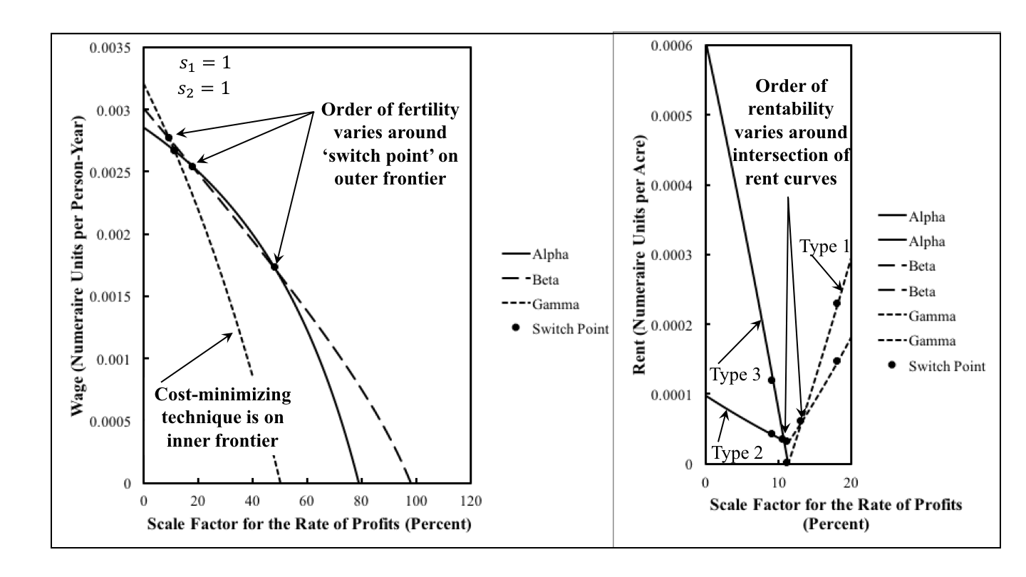
Figure 2 illustrates wage and rent curves when s₁ and s₂ are unity. Markets are competitive, and the scale factor for the rate of profits is merely the rate of profits. The cost-minimizing technique corresponds to the wage curve on the inner frontier.

Consider a rate of profits of zero or just barely positive. Alpha is cost-minimizing. If the requirements for use were small enough that they could be satisfied by only farming Type 3 land, a technique with same wage curve as Gamma would be cost-minimizing. No land would pay rent and the wage would be as shown on the highest wage curve. With somewhat greater requirements for use, Type 2 land would be taken into cultivation, and the wage would be as shown on the wage curve for Beta. Type 3 land would be fully cultivated and pay a rent. Finally, with the originally postulated requirements for use, Type 1 land is cultivated. In the range for the smallest rate of profits, the order of fertility, from most fertile to least fertile land, is Type 3, Type 2, Type 1.

Figure 2: Wage and Rent Curves with Competitive Markets

Alpha is still cost-minimizing for a rate of profits greater than that at the first intersection on the outer frontier for the wage curves, but smaller than that at the switch point on the inner frontier of the wage curves. For a given rate of profits the order of fertility is from the type of land associated with the technique with the highest wage curve downwards. In this range of the rate of profits, the order of fertility is Type 2, Type 3, Type 1.

This is an example of the reswitching of the order of fertility. When Gamma is cost-minimizing, the order of fertility varies from Type 2, Type 1, Type 3 lands to Type 1, Type 2, Type 3 lands and back. The wage curve for the Beta technique is never on the inner frontier, and Beta is never cost-minimizing.

Rent curves are graphed on the right pane in Figure 2. For each switch point for the wage curves, a pair of points, vertically stacked, are shown on the graph of rent curves. For the switch points on the inner frontier of the wage curves, two rent curves intersect at a rent of zero. Type 1 and Type 3 lands pay no rent at this switch point. The switch points for the intersections on the outer frontier of wage curves are not striking on the graph of the rent curves.

The intersections for the rent curves occur at rates of profits different from those for which wage curves intersect. When Alpha is cost-minimizing, the order of rentability varies from Type 3, Type 2, Type 1 to Type 2, Type 3, Type 1. The order of fertility first matches the order of rentability, then deviates from it at a higher rate of profits, then matches again at a still higher rate of profits. Whether or not the orders of fertility and rentability match also varies with the rate of profits in the range where Gamma is cost-minimizing and Type 3 land pays no rent.

Figure 3: Distribution of National Income with Competitive Markets

Given net output and the rate of profits, the levels of operation of each process, the prices of their inputs, and the value of the components of net output are defined. Figure 3 plots total wages, rent, and profits as functions of the rate of profits. Since net output is taken as numeraire, these components add up to unity, whatever the rate of profits. Wages decrease and profits increase with the rate of profits, but rents do not vary monotonically. When Type 1 land is non-scarce, total rents decrease with the rate of profits. When Type 3 land is non-scarce, on the other hand, total rents increase with the rate of profits.

5.0 Perturbing Relative Markups

The non-competitive case can differ qualitatively from the competitive case presented in Section 4. In a non-competitive case, with agriculture having sufficient market power, Beta is sometimes cost-minimizing. This is never so in the competitive case. Throughout the range for the scale factor for the rate of profits in which the Alpha technique is cost-minimizing in this non-competitive case, the orders of efficiency and rentability do not vary. The same is true for the range of the scale factor in which Gamma is cost-minimizing. The opposite is true in the competitive case, and sometimes the order of rentability does not match the order of fertility when Alpha or Gamma are cost-minimizing.

One can construct an overall picture of how these changes come about by analyzing the full range of possible ratios of the markup in industry to the markup in agriculture. The heavy, solid lines in Figure 1, at the top of this post, are switch points on the inner frontier of the wage curves and the maximum scale factor for the rate of profits. The cost-minimizing technique is labeled. The dashed lines are intersections on the outer frontier of the wage curves. The order of fertility varies across dashed lines. Dotted lines are intersections of rent curves. The order of rentability varies across dotted lines. Dashed lines are hard to perceive to the right, when industry has more market power than agriculture.

Figure 4: Enlargement of Variation with Relative Markups

Thin vertical lines partition the axis for the ratio of markups. Each vertical line corresponds to a fluke case. Figure 4 enlarges the left part of the figure, where agriculture has the most market power. For the first fluke case, the rent curves for Type 1 and Type 3 lands, when Beta is cost-minimizing, become tangent at the indicated ratio of markups. The partition between the second and third region is a fluke case where the second intersection for the rent curves for Type 1 and Type 3 lands occurs at the maximum value for the scale factor for the rate of profits. At the ratio for markups for the third fluke case, the wage curves for Beta and Gamma techniques intersect with a wage of zero. The fourth fluke case is a ratio of markups such that all three wage curves intersect at a single switch point. The rents of all three types of land are zero at that switch point. The fifth fluke case, at a partition between Regions 5 and 6, is such that the wage curves for Alpha and Beta intersect at the maximum scale factor for the Gamma technique. The wage curves for the Alpha and Beta techniques are tangent at a switch point for the ratio of markups at the last fluke case.

Table 3 summarizes this numeric example. Variations in the cost-minimizing technique, in the order of fertility, and in the order of rentability with the scale factor for the rate of profits are indicated. In Region 1, agriculture has the most extreme level of market power over industry. The wage curve for Alpha intersects the wage curve for Beta on the inner frontier and then the wage curve for Gamma on the outer frontier. The rent curves do not intersect in the appropriate ranges of the scale factor for the rate of profits. The order of rentability only varies with the cost-minimizing technique.

Table 3: Variations in the Cost-Minimizing Technique

Region	Range	Technique	Order of Fertility	Order of Rentability
1	0 ≤ r ≤ r1	Alpha	Type 3, 2, 1	Type 3, 2, 1
	r1 ≤ r ≤ r2	Beta	Type 3, 1, 2	Type 3, 1, 2
	r2 ≤ r ≤ rmax, β		Type 1, 3, 2
2	0 ≤ r ≤ r1	Alpha	Type 3, 2, 1	Type 3, 2, 1
	r1 ≤ r ≤ r2	Beta	Type 3, 1, 2	Type 3, 1, 2
	r2 ≤ r ≤ r*		Type 1, 3, 2
	r* ≤ r ≤ r**			Type 1, 3, 2
	r** ≤ r ≤ rmax, β			Type 3, 1, 2
3	0 ≤ r ≤ r1	Alpha	Type 3, 2, 1	Type 3, 2, 1
	r1 ≤ r ≤ r2	Beta	Type 3, 1, 2	Type 3, 1, 2
	r2 ≤ r ≤ r*		Type 1, 3, 2
	r* ≤ r ≤ rmax, β			Type 1, 3, 2
4	0 ≤ r ≤ r1	Alpha	Type 3, 2, 1	Type 3, 2, 1
	r1 ≤ r ≤ r2	Beta	Type 3, 1, 2	Type 3, 1, 2
	r2 ≤ r ≤ r*		Type 1, 3, 2
	r* ≤ r ≤ r3			Type 1, 3, 2
	r3 ≤ r ≤ rmax, γ	Gamma	Type 1, 2, 3	Type 1, 2, 3
5	0 ≤ r ≤ r1	Alpha	Type 3, 2, 1	Type 3, 2, 1
	r1 ≤ r ≤ r*		Type 2, 3, 1
	r* ≤ r ≤ r2			Type 2, 3, 1
	r2 ≤ r ≤ r**	Gamma	Type 2, 1, 3	Type 2, 1, 3
	r** ≤ r ≤ r3			Type 1, 2, 3
	r3 ≤ r ≤ rmax, γ		Type 1, 2, 3
6	0 ≤ r ≤ r1	Alpha	Type 3, 2, 1	Type 3, 2, 1
	r1 ≤ r ≤ r*		Type 2, 3, 1
	r* ≤ r ≤ r2			Type 2, 3, 1
	r2 ≤ r ≤ r**	Gamma	Type 2, 1, 3	Type 2, 1, 3
	r** ≤ r ≤ r3			Type 1, 2, 3
	r3 ≤ r ≤ r4		Type 1, 2, 3
	r4 ≤ r ≤ rmax, γ		Type 2, 1, 3
7	0 ≤ r ≤ r1	Alpha	Type 3, 2, 1	Type 3, 2, 1
	r1 ≤ r ≤ r*		Type 2, 3, 1
	r* ≤ r ≤ r2			Type 2, 3, 1
	r2 ≤ r ≤ r**	Gamma	Type 2, 1, 3	Type 2, 1, 3
	r** ≤ r ≤ rmax, γ			Type 1, 2, 3

Region 2, and the fluke cases bounding it, illustrates that a persistent change in the relative market power among industries can bring about the reswitching of the order of rentability. The rent curves for Type 1 and Type 3 land intersect twice in the range of the scale factor of profits in which Beta is cost-minimizing. The rent curves for both types of land are increasing functions of the scale factor in this range.

The rent curve for Type 3 land becomes downward-sloping in Region 3. It is not always monotone. The order of rentability at the highest range of the scale factor for the rate of profits in Region 2 has disappeared in Region 3. With some thought, one can see how the variations between regions in the ranges of the scale factor for the cost-minimizing technique, the order of fertility, and the order of rentability relate to the fluke cases dividing these regions. The range of the scale factor in which Beta is cost-minimizing has disappeared in Region 5, after the switch point at which all three wage curves intersect. Switch points between Alpha and Beta and between Beta and Gamma are thenchforth on the outer wage frontier and are the occasion of a change in the order of fertility. Region 6 is an example of the reswitching of the order of fertility, and is illustrated in Section 4 with the competitive case. In Region 7, the last in the table, the order of fertility does not vary when Gamma is cost-minimizing.

6.0 Conclusion

The numerical example illustrates complications that can arise in the conflict over the distribution of the surplus among workers, capitalists in various industries, and owners of types of land. I take the coefficients of production as frozen in considering this conflict. That is, I do not consider the conflict over the length of the working day, the intensity with which workers work, the care they must take to prevent waste, the right to urinate on the job, and so on. Nor do I consider some conflicts between capitalists and landlords, outside of distribution. For example, landlords would like leases as short as possible so as to be able to raise rents for more-or-less permanent improvements brought about by the capitalists, while the capitalists would like longer rents to prevent this outcome.

The model illustrated above is one in which relative markups are given. It demonstrates that in the competitive case, the order of fertility of lands can vary with the rate of profits, where the rate of profits is taken as given from outside the model. The order of fertility can vary both with and without the cost-minimizing technique varying. The order of lands from high rent to low rent lands also varies, in general, with the rate of profits. One may find that ownership of one type of asset provides greater returns than another, even though the latter asset is more efficient at the going rate of profits.

Persistent differences in markups among industries does not alter these conclusions, but does provide the possibility of qualitative and quantitative variation in details. In the example, if agriculture has sufficient market power over industry, the example no longer exhibits a reswitching of the order of fertility. A range of the scale factor for the rate of profits emerges in which type 2 land no longer obtains a rent. An even further increase in the market power of agriculture can lead to the appearance and the disappearance of the reswitching of the order of rentability

No simple picture emerges from this analysis. The workers can only obtain a larger share of the surplus product if the capitalists get less. Whether or not the landlords are able to obtain a larger share with either an increased rate of profits or increased market power for some sectors varies