A Switch Point Without Intersecting Wage Curves

Figure 1: Start of Wage Curves, with One Real and One Fake Switch Point

1.0 Introduction

This post presents another numeric example with pure fixed capital and extensive rent. Aside from these aspects of the model, no joint production exists.

Models of pure fixed capital or of extensive rent share certain properties with models of the production of commodities with labor and circulating capital alone. This article demonstrates that a model that combines pure fixed capital and extensive rent can exhibit issues raised by joint production. The cost-minimizing technique need not maximize the wage, and the choice of technique cannot be analyzed by the construction of the wage frontier. A switch point can exist without an intersection of wage curves, and intersections of wage curves can be fake switch points.

2.0 Technology

The example is specified by the technology, endowments of land, and requirements for use. An analysis of quantity flows identifies which techniques are feasible at a given level of requirements for use. The analysis of the choice of technique requires the examination of the solutions to the price systems for each technique.

I assume the existence of two types of land. More than one type is required for this model to exhibit extensive rent. With only two types of land, contrasting the orders of efficiency and of rentability is uninteresting. The order of efficiency is the order in which different types of land are introduced into cultivation as net output expands. The order of rentability sorts the lands by rent per acre. When both types of land are farmed, one type will be only partially farmed. It has a rent of zero; the other type of land obtains a positive rent. The orders of efficiency and rentability are necessarily identical, with two types of land and only one scarce. These orders can be completely reversed in models with more lands and both extensive and intensive rent.

Fixed capital is another aspect of joint production, in addition to land, in this model. A newly produced machine can be used for three years in production. Machines are assumed not to be consumption goods. New machines, but not old machines, can be consumer goods in models of pure fixed capital. This model seems to be close to the minimal complexity to investigate a combination of land-like natural resources and fixed capital in a model with the production of multiple commodities that is otherwise of single production alone. In a simpler model, the physical life of the machine would be only two years.

Table 1: Inputs for Processes Comprising the Technology

Input	Processes
	I	II	III	IV	V	VI	VII
Labor	a0,1 = 0.4	a0,2 = 0.2	a0,3 = 0.6	a0,4 = 0.4	a0,5 = 0.23	a0,6 = 0.59	a0,7 = 0.39
Type 1 Land	0	c1,2 = 1	c1,3 = 1	c1,4 = 1	0	0	0
Type 2 Land	0	0	0	0	c2,5 = 1	c2,6 = 1	c2,7 = 1
Corn	a1,1 = 0.1	a1,2 = 0.4	a1,3 = 0.578	a1,4 = 0.6	a1,5 = 0.39	a1,6 = 0.59	a1,7 = 0.61
New Machines	0	1	0	0	1	0	0
Type 1 1-Yr. Old Machines	0	0	1	0	0	0	0
Type 1 2-Yr. Old Machines	0	0	0	1	0	0	0
Type 2 1-Yr. Old Machines	0	0	0	0	0	1	0
Type 1 2-Yr. Old Machines	0	0	0	0	0	0	1

The technology is specified by the coefficients of production for seven processes. Each column in Table 1 shows the person-years of labor, acres of either type of land, bushels of corn, and numbers of new and old machines required as inputs to operate a process at unit level. The outputs of corn and machines, new and old, per unit level of each process are shown in Table 2. Machines are an industrial product which needs no land to produce. The laborers produce corn on land from inputs of corn and machines. Old machines one year older are produced jointly with corn from inputs of machines. Each old machine is of a type customized to the land on which it was produced. Old machines cannot be transferred from one type of land to another. They are assumed to be capable of free disposal. Formally, free disposal of an old machine of, say, type 1 is specified by assuming the existence of another process duplicating the second or third process, but without an output of an old machine. Each process is assumed to exhibit constant returns to scale (CRS) and to require a year to complete. The coefficients of production for the first four processes, other than those for land, are taken from a reswitching example by Baldone (1980).

Table 2: Outputs for Processes Comprising the Technology

Input	Processes
	I	II	III	IV	V	VI	VII
Corn	0	b1,2 = 1	b1,3 = 1	b1,4 = 1	b1,5 = 1	b1,6 = 1	b1,7 = 1
New Machines	1	0	0	0	0	0	0
Type 1 1-Yr. Old Machines	0	1	0	0	0	0	0
Type 1 2-Yr. Old Machines	0	0	1	0	0	0	0
Type 2 1-Yr. Old Machines	0	0	0	0	1	0	0
Type 1 2-Yr. Old Machines	0	0	0	0	0	1	0

The specification of model parameters is completed with endowments and requirements for use. Assume 100 acres of each type of land exist. The required net output is assumed to be 87 bushels corn. This required net output is such that all and only the techniques which require both types of land to be farmed are feasible.

3.0 Techniques and Feasibility

A technique is defined by which processes are operated, which type of lands are left unfarmed, which are partially farmed, and which are farmed to the full extent of their endowment. Rents can only be obtained on the last. Twenty-four techniques (Table 3) are defined for this technology. The capital goods that are used up in operating a technique can be reproduced. A net output remains, consisting, in the example, solely of corn.

Only scarce lands obtain a rent, and which are scarce varies with the technique. No land is scarce in the Alpha through Zeta techniques. One land is farmed and not to its full extent. Type 1 land is scarce in the Eta through Omicron techniques, while type 2 land is scarce in the remaining nine techniques. The techniques also vary in the economic life of the machine, one, two, or three years, on each type of land. Under the assumptions, the first six techniques are infeasible. Only Eta through Omega are feasible.

Table 3: Techniques of Production

Technique	Processes	Type 1 Land	Type 2 Land
Alpha	I, II	Partially farmed	Fallow
Beta	I, II, III	Partially farmed	Fallow
Gamma	I, II, III, IV	Partially farmed	Fallow
Delta	I, V	Fallow	Partially farmed
Epsilon	I, V, VI	Fallow	Partially farmed
Zeta	I, V, VI, VII	Fallow	Partially farmed
Eta	I, II, V	Fully farmed	Partially farmed
Theta	I, II, III, V	Fully farmed	Partially farmed
Iota	I, II, III, IV, V	Fully farmed	Partially farmed
Kappa	I, II, V, VI	Fully farmed	Partially farmed
Lambda	I, II, III, V, VI	Fully farmed	Partially farmed
Mu	I, II, III, IV, V, VI	Fully farmed	Partially farmed
Nu	I, II, V, VI, VII	Fully farmed	Partially farmed
Xi	I, II, III, V, VI, VII	Fully farmed	Partially farmed
Omicron	I, II, III, IV, V, VI, VII	Fully farmed	Partially farmed
Pi	I, II, V	Partially farmed	Fully farmed
Rho	I, II, III, V	Partially farmed	Fully farmed
Sigma	I, II, III, IV, V	Partially farmed	Fully farmed
Tau	I, II, V, VI	Partially farmed	Fully farmed
Upsilon	I, II, III, V, VI	Partially farmed	Fully farmed
Phi	I, II, III, IV, V, VI	Partially farmed	Fully farmed
Chi	I, II, V, VI, VII	Partially farmed	Fully farmed
Psi	I, II, III, V, VI, VII	Partially farmed	Fully farmed
Omega	I, II, III, IV, V, VI, VII	Partially farmed	Fully farmed

4.0 The Price System

The modeled economy consists of three classes: workers, landlords, and capitalists. Capitalists buy inputs and hire workers who they direct to produce commodity outputs. In agriculture, capitalist farmers pay rent on scarce land to landlords. The capitalists choose the processes to operate based on cost. Accordingly, prices must be analyzed.

A system of equations is associated with each technique. An equation characterizes the prices for each process operated under a technique. These equations show the same rate of accounting profits is obtained on the value of the capital goods advanced at the start of the year. Rent and wages are paid out of the surplus product at the end of the year. A bushel corn is numeraire. The rent per acre appears in the equation for processes operating on the land that is fully farmed, if any. This land is scarce. Lands that are not fully farmed are free, and no rent appears in the equations for the processes operating on them.

5.0 On the Solutions of the Price Systems

Given the rate of profits, the price system for each technique can be solved. The solution for a technique has one degree of freedom. The solution can be presented with the wage, the price of new and old machines, and rents per acre as functions of the rate of profits. Figure 1 graphs the start of the wage curves for each technique in the example. Notice that the ordinate does not begin at zero in the graph. In this example, each wage curve is downward-sloping. Wage curves can be upward-sloping off the outer wage frontier in models of fixed capital. In this example with fixed capital and extensive rent, the wage frontier is neither the outer frontier of all wage curves nor the inner frontier.

In the illustrated range of the rate of profits, the wage frontier is the wage curve for the Zeta, Nu, Xi, and Omicron techniques. The wage curve for a technique is found from solving the price system formed from the machine-building process and the corn-producing processes operating on the non-scarce type of land. Quadrio Curzio & Pellizzari (2010) call this the ‘solving subsystem’. The Zeta, Nu, Xi, and Omicron techniques differ on which processes are operated on Type 1 land, but not on Type 2 land, which is free for all four techniques. Thus, they have the same solving system and the same wage curve.

Why are the wage curves for Nu and Omicron cost-minimizing in the illustrated range of the rate of profits? A technique is cost-minimizing at a given rate of profits if:

• The wage and the prices of all produced commodities (corn and machines of various types and vintages) are positive.
• The rent of the scarce type of land is positive.
• The prices of old machines not produced by the technique are negative for the price systems in which they are produced. Bidard (2016) defines ghost commodities as such non-produced commodities that affect the prices of produced commodities.

The price of a Type 1 old machine is negative under Omicron prices for rates of profits smaller than at the switch point between Nu and Omicron. A more general model would have processes that do not result from extending the economic life of a machine produced by the technique under consideration. For the technique to be cost-minimizing, no extra profits can be obtained by operating additional processes at the prices for the given rate of profits.

Two techniques are cost-minimizing at a switch point, except in fluke cases. The wage and the prices of all commodities produced with both techniques do not vary between the price systems for the two techniques. The rent per acre of land is also the same for the two techniques cost-minimizing at a switch point. Two types of switch points exist in the example, in addition to fake switch points.

In the first type, the techniques that are cost-minimizing for a switch point differ in the economic life of a machine. For example, the economic life of a machine used in farming Type 1 land is one year under Nu and three years under Omicron. Figure 2 illustrates the switch point between Nu and Omicron. Gamma, Sigma, Phi, Omega, Iota, Mu, and Omicron have positive prices for Type 1 one-year old machines in the graphed ranges of the rate of profits. Type 1 one-year old machines are also produced in the Beta, Rho, Upsilon, Psi, Theta, Lambda, and Xi techniques. Their prices are negative for these techniques in the indicated range. The price is zero, at the switch point, of the machine one year older than used in the technique with the shorter life in the price system for the other technique. A price of zero is a signal that the economic life of the machine can be truncated.

Figure 2: Price of Type 1 One-Year-Old Machines (Detail)

Rents per acre are zero at the other type of switch point. In the example, a switch point between Iota and Sigma exists at a rate of profits of approximately 45.04 percent. Their wage curves intersect at the switch point. The machine is run for its full physical life on Type 1 land under both techniques, and truncated after its first year of operation on Type 2 land. The techniques differ in which type of land is fully farmed and which is free. Figures 3 and 4 depict the rent curves for the example. The rent curve for Iota intersects the abscissa in Figure 3. Type 1 land is free under Sigma and has a rent per acre of zero under Iota at the switch point. Likewise, the rent curve for Sigma intersects the abscissa at the switch point in Figure 4. The rent per acre on Type 2 land is zero at the switch point.

Figure 3: Rent On Type 1 Land

Figure 4: Rent On Type 2 Land

A fluke switch point in which four techniques are cost-minimizing can combine these two types of switch points. Two techniques can differ in both the economic life of a machine and in which land is fully farmed. Two other techniques would then be cost-minimizing so that firms are indifferent between the economic life of the machine and which land is fully farmed. Two of these four techniques would differ in the economic life of a machine on scarce land; they would have the same wage curve. A switch point in which both the economic life of a machine and which type of land is scarce vary is the intersection of three wage curves.

Fake switch points arise when only two wage curves intersect for techniques which vary in both the economic life of a machine and the type of land that is fully farmed. Two fakes (Table 4) appear in the example. In both fakes, the prices of commodities produced under both techniques with intersecting wage curves do not vary between the techniques. For the first fake, the technique Omicron with the longer economic life of a machine is cost-minimizing. For the second fake, the technique Lambda with the longer economic life of a machine is not cost-minimizing. No price of these commodities not produced under both techniques are not zero under the technique in which they are produced. Their prices deviate from their behavior under the first type of switch point described above. On the other hand, the rent of one type of land, Type 2 for the first fake and Type 1 for the second, is zero for both techniques, as in the second type of switch point. The rent on the other type of land is positive for the technique for which it is scarce. The first switch point is a fake because the wage curve for Omega does not intersect with the other wage curves. Under Omicron and Omega, the economic lives of the machines are the same. The techniques differ in which land is scarce. By the same logic, the wage curve for Theta must intersect at the second switch point in Table 5 for it not to be a fake.

Table 4: Rent Per Acre Varies with the Technique at Fake Switch Points

Rate of Profits (Percent)	Technique	Commodities Produced Under Both	Ghost Commodities	Type 1 Land	Type 2 Land
15.9	Omicron*	Corn, New machines, Type 2 one and two-year old machines.	Type 1 one and two-year old machines. Prices of both are positive.	Scarce. Rent is positive.	Free
	Chi	Prices are positive and same as Omicron.		Free	Scarce. Rent is positive.
56.7	Lambda	Corn, new machines, Type 1 one-year old machines.	Type 1 one and two-year old machines. Prices of both are positive.	Scarce. Rent is positive.	Free
	Rho*	Prices are positive and same as Lambda.		Free	Scarce. Rent is positive.

6.0 The Cost-Minimizing Systems

A numeric example that combines the production and use of fixed capital with extensive rent is developed above. Table 5 summarizes the variation in the cost-minimizing technique through the full range of the rate of profits. The boundaries on the ranges at which techniques are cost-minimizing are approximate. The switch point between Pi and Rho exhibits capital-reversing. A higher wage or lower rate of profits is associated with the adoption of a technique that requires greater employment per unit of net output. This result is a challenge for what some obdurate economists still teach, that, under ideal assumptions, equilibria in the labor market must be the intersections of well-behaved, monotonic supply and demand curves. These results are also a challenge for claims by economists of the Austrian school. For the switch points between Iota and Omicron and between Rho and Sigma, a longer economic life of a machine is associated with greater capital-intensity, as they would expect. But for the switch points between Nu and Omicron and between Pi and Rho, a shorter economic life of a machine is associated with greater capital-intensity

Table 5: Cost-Minimizing Techniques

Range (Percent)	Technique	Economic Life of Machine (Years)		Land
		Type 1	Type 2	Type 1	Type 2
0 ≤ r ≤ 5.12	Nu	1	3	Scarce	Free
5.12 ≤ r ≤ 36.3	Omicron	3	3	Scarce	Free
36.3 ≤ r ≤ 45.0	Iota	3	1	Scarce	Free
45.0 ≤ r ≤ 55.7	Sigma	3	1	Free	Scarce
55.7 ≤ r ≤ 62.7	Rho	2	1	Free	Scarce
62.7 ≤ r ≤ 74.2	Pi	1	1	Free	Scarce

7.0 Conclusions

Joint production presents the possibilities of many phenomena inconsistent with clear properties of models of the production of commodities with circulating capital alone. This article demonstrates that at least some of these phenomena can occur with the combination of fixed capital and extensive rent, even though they do not occur in models of pure fixed capital and extensive rent considered separately. The choice of technique cannot be analyzed solely by the construction of the wage frontier. A switch point exists at which two wage curves do not intersect. Two fake switch points exist in the example, where rents per acre are not equal on one type of land at the switch point for the techniques with intersecting wage curves. The feasible technique with the largest wage is not necessarily cost-minimizing

No claim is made that other issues of joint production might not arise in models combining fixed capital and extensive rent. D’Agata (1983) provides an example in a model of intensive rent with a non-unique and sometimes upward-sloping wage frontier. The model in this article is similar to a model of intensive rent in some ways. Can an example be given with these properties?

A model with more types of land provides a setting for comparing and contrasting the orders of efficiency and rentability. The analysis in this article demonstrates that the wage frontier for cost-minimizing techniques is disconnected from the ordering of wage curves. How does the order in which lands are introduced into cultivation, at a given rate of profits, relate to the ordering of wage curves in models with fixed capital? Presumably, the introduction of fixed capital still allows for the order of rentability to differ from the order of efficiency. More efficient lands are not necessarily paid a higher rent per acre.

Models of rent emphasize the need to consider technical change. Net output can be increased only up to a hard limit. The introduction of new processes and techniques, a capability to extend the physical life of machines, the discovery of new natural resources, or decreases in some coefficients of production for existing processes are required to increase net output beyond that limit. Introduction of such possibilities into the model will result in structural economic dynamics.

CCC: tl; dr

1.0 Introduction

You can easily find peopole on the Internet asking for a summary of the Cambridge Capital Controversy. An answer is easy.

Supply and demand is balderdash. If you want to understand markets under capitalism, you might as well throw away most microeconomic textbooks and most introductory textbooks.

2.0 Some Expansions

No consistent, valid model in which more than one commodity is produced supports the following two mistaken stories.

Suppose the tastes of those making decisions for households change. They become more future-oriented, more willing to defer consumption. The supply of capital has increased. With an increased supply, the interest rate is driven down. The firms ultimately choose to adopt more capital-intensive techniques. They tend to equip workers with more machinery and to run exisiting machinery longer.

Suppose, again, that the tastes of those making decisions for households change. Workers now prefer consumption over leisure more than they did before. The supply of labor has increased. The real wage is driven down. Firms ultimately choose to adopt more labor-intensive techniques. Equilibrium employment in competitive markets thereby increases.

Numerical examples of capital-reversing and other so-called capital-theoretical paradoxes or perversities are enough to demonstrate that the above stories do not follow from the assumptions of mainstream economics.

3.0 Extension to Technical Discussions

Well-educated economists know that their theory does not support the causal stories in the textbooks. I concentrated above on factor markets. I now go into more technical points. I think that if my powers of exposition and understanding were much greater, this section would still not be clear.

The above refuted stories can be augmented with stories about natural resources and about produced commodities. The assumptions of mainstream economics do not justify explaining equilibrium by the intersection of well-behaved supply and demand curves.

Demonstrations of capital-reversing, for example, are usually presented in open models of competitive, cost-minimizing firms. These models can be closed by assuming households are utility-maximizing. These closures include intertemporal utility-mximizing. Overlapping generations (OLG) models are examples.

Are long-run equilbrium models like this 'neoclassical'? Endowments of capital are not among the givens. The mixture and level of capital goods are found from solving the model. Likewise, the numeraire value of the capital stock is endogeneous, not a parameter.

The claim that, in equilibrium, the rate of interest is equal to the marginal product of capital might be justified as applying to Champernowne's chain index measure of the quantity of capital. This chain index, basically, excludes price Wicksell effects from the measure of the quantity of capital. Both the interest rate and the value of this chain index are found from the solution of the model. They are not part of what needs to be known to find the solution. Furthermore, the chain index is not what is measured in empirical applications of the Solow-Swan model and in measurements of total factor productivity (TFP).

Another argument turns around how capital-theory paradoxes apply to models of intertemporal equilibria, if at all. Can a continuum of equilibria be found in either long-run models or models of intertemporal equilibrium? Do capital-theoretic paradoxes add anything to examination of the stability of intertemporal equilibrium, either for tattonement or for individual paths? Typically, stability cannot be demonstrated, and multiple equilibria exist. No reason exists to expect paths to approach steady states. J. Barkley Rosser Jr. argued that the reswitching of techniques is manifested in intertemporal equilibrium as a cusp catastrophe. Personnally, I think Michael Mandler is more correct than Pierangelo Garegnani about stability.

I finally bring up that you do not have to close long run models with intertemporal utility-maximization. Richard Kahn, Nicholas Kaldor, Luigi Pasinetti, and Joan Robinson had closures related to the Cambridge equation. Or you can take the wage as a matter of social conventions or norms. Or, perhaps, you can have a monetary theory of distribution, in which the monetary authority sets the interest rate. Stephen Marglin had a overdetermined closure that explained stagflation. Questions exist about how some of these closures relate to a generalization of John Maynard Keynes' principle of effective demand to the long run.

I see I have left out debates over the the history of more than two centuries of political economy.

4.0 Conclusion

But the mainstream defenders in these discussion are not defending what is in the textbooks. The simple-minded depiction of well-behaved supply and demand curves determining equilibrium lacks any theoretical or empirical foundation.

Recurrence Of Truncation Without Reswitching

Figure 1: Wage Curves In The Example

1.0 Introduction

I have presented this example before. This example is another case of exploring or demonstrating code written for Matlab or Octave.

The structure of the example is the minimum multi-industry example with circulating and fixed capital in all industries and in which the choice of technique is to select the economic life of a machine.

The recurrence of truncation is like the recurrence of a process in single production. As far as I know, no numeric example exists in the literature of the recurrence of truncation without reswitching. This example might have been surprising if I were writing half a century ago. Its possibility is obvious in the work of Bertram Shefold, Heinz Kurz & Neri Salvadori, Ian Steedman, and others. Although reswitching and capital-reversing do not arise in the example, the reverse substitution of labor does.

2.0 Technology and Techniques

Two industries exist in the example. One industry produces machines, and the other industry produces corn. Corn is a consumption good, the good for circulating capital, and the numeraire. Machines are fixed capital. Each machine has a physical life of two years. Old machines cannot be transferred between industries. I assume constant returns to scale (CRS) and the free disposal of old machines. Labor is advanced and paid out of the surplus of corn.

Tables 1 and 2 show the inputs and outputs for each process known to the managers of firms. For example, the inputs, at a unit level of operation, consist of 1/10 person-years, 1/16 bushels corn, and one new machine. The outputs, available after a year, are two new machines and one machine a year older.

Table 1: Inputs for The Technology

Input	Industry
	Machine		Corn
	I	II	III	IV
Labor	1/10	8	43/40	1
Corn	1/16	3/20	1/8	53/200
New Machines	1	0	1	0
One-Year Old Machines (1st type)	0	1	0	0
One-Year Old Machines (2nd type)	0	0	0	1

Table 2: Outputs for The Technology

Output	Industry
	Machine		Corn
	I	II	III	IV
Corn	0	0	1	14/25
New Machines	2	5/2	0	0
One-Year Old Machines (1st type)	1	0	0	0
One-Year Old Machines (2nd type)	0	0	1	0

The machines operate an non-constant efficiency in both industries. An old machine, in the machine industry, is used to produce more new machines than a new machine. The inputs of labor services and corn increase with the age of the machine. In the corn industry, an ole machine is used to produce less corn than a new machine. The input of labor services decrease and the corn input increases with the age of the machine.

With this specification of the technology, the economic life of the machine must be chosen in each industry. Table 3 lists the available techniques. The machine is truncated in both industries in the Alpha technique. The machine is operated for its full physical life in both industries in the Delta technique. In Beta and Gamma, the machine is truncated in one industry and operated for its full physical life in the other.

Table 3: Specification of Techniques

Technique	Processes
Alpha	I, III
Beta	I, II, III
Gamma	I, III, IV
Delta	I, II, III, IV

3.0 Price Systems and the Cost-Minizing Technique

The economic life of a machine is chosen to minimize cost. A system of equations for prices is associated with each technique. This system can be solved. In the solution, the wage is a function of the rate of profit. Each price of a produced commodity is also a function of the rate of profits.

Figure 1 shows the wage curves, for the four techniques in the example. The cost-minimizing technique at each wage or rate of profits is the technique with its wage curve on the outer frontier. The cost-minimizing techniques are indicated on the figure. Maybe I should experiment with perturbing parameters to see if I can get a more visually obvious graph. Figure 2 shows an enlargement, emphasizing rates of profits around the switch point between Gamma and Delta.

Figure 2: Wage Curves In The Example (Enlarged)

At any rate, the cost-minimizing techniques, in order of an increasing rate of profits, are Alpha, Gamma, Delta, and Beta. Each pair of techniques at a switch point on the frontier differs in one process. A switch point in which the economic life of a machine differs in both industries would be a fluke case. No fluke switch points exist in this example, without perturbing some coefficients of production.

4.0 Prices of Old Machines

Identifying when prices of old machines are negative provides another method of analyzing the choice of technique in models of pure fixed capital. A negative price indicates that the economic life of a machine should be shortened. The machine should be truncated and discarded.

Figure 3 plots the price of old machines in the machine industry, for the two techniques in which old machines are operated in this industry. The switch points, at which the price of an old machine is zero, are indicated. As can be seen in Figure 2, the switch point between Alpha and Beta is not on the outer frontier.

For rates of profits less than that at the switch point between Gamma and Delta, the price of an old machine in the machine industry is negative for the Delta price system. If the Delta technique were in operation, prices would signal that machines in the Delta industry should be truncated. This trunction results in the Gamma tecnique being adopted.

Figure 3: The Price of an Old Machine in Machine Production

Figure 4 plots the price of old machines in the corn industry. Old machines are operated in this industry only for Beta and Delta. Since the price of these old machines are negative, in the Gamma price system, for rates of profits less than the rate at which the price is zero, the machine is truncated at these rates and the Alpha technique is adopted. Likewise, at rates of profits greater than the rate at which the price of this machine is zero, in the Delta system, the machine is truncated and the Beta technique is cost-minimizing at these rates.

Figure 4: The Price of an Old Machine in Corn Production

This analysis of prices of old machines has re-justified the analysis of the choice of technique in Section 4.

5.0 Extra Profits in Extending the Economic Life of Machines

A third method of examining the choice of technique is available.

Under Alpha and Gamma, the machine is truncated in the machine industry. The price of an old machine in the machine industry is zero under those price systems. Figure 5 shows extra profits, for each technique, available in operating the machine for a second year. if the life of this type of machine is extended under Gamma, the Delta technique is adopted. Extra profits are available in so extending the life of the machine at any rate of profits greater than at the switch point between Gamma and Delta. Gamma cannot be cost-minimizing in this range.

Figure 5: Extra Profits in the Machine Industry

The machine is truncated in the corn industry for Alpha and Beta. Figure 6 shows extra profits in the corn-industry, for all techniques, in operating the machine for a second year. Extra profits cannot be obtained for Alpha up to the switch point between Alpha and Gamma. Likewise, extra profits are not available for Beta, in extending the life of the machine in corn-production, for rates of profits greater than at the switch point between Beta and Delta. This method of analyzing the choice of technique, not surprisingly, yields the same result as the other two.

Figure 6: Extra Profits in the Machine Industry

6.0 Recap

The above has illustrated three equivalent methods of analyzing the choice of technique for a pure fixed capital model. Table 4 summarizes the results for this numerical example. The bounds on the ranges of the rates of profits are approximate. Matlab has a funtion, roots(), that returns the (possibly complex) zeros for a polynomial of any degree. I use this function in finding the intersections of wage curves in this example.

Table 4: Cost-Minimizing Techniques

Range	Technique	Truncation
0 ≤ r ≤ 70.21%	Alpha	Machines truncated in both industries.
70.21% ≤ r ≤ 71.19%	Gamma	Machines truncated in machine-production.
71.19% ≤ r ≤ 87.5%	Delta	Machines operated at full physical life in both industries.
87.5% ≤ r ≤ 122.8%	Beta	Machines truncated in corn-production.

At any rate, the machine is truncated in corn-production when both the Alpha and the Beta technique are cost-minimizing. The truncation of the machine in corn-production recurs, being part of the cost-minimizing technique at extremes of low and high rates of profits. This is not, however, an example of the reswitching of techniques.

Negative real Wicksell effects occur at all four switch points. Around each switch point, a lower rate of profits and higher wage is associated with a greater net output of corn per person-year. At the switch point between Alpha and Gamma, truncation in the corn industry is a switch to a more capital-intensive technique. Likewise, at the switch point Gamma and Delta, truncation in the machine industry is a switch to a more capital-intensive technique. As usual, these results disagree with Austrian capital theory and the ideas of economists of this school about roundaboutness.

Around the switch point between Alpha and Gamma, a lower rate of profits or higher wage is associated with truncation in the corn industry and a greater gross output of corn per person-year hired in the corn industry. Around the switch point between Delta and Beta, contrawise, a lower rate of profits or higher wage is associated with the extension of the economic life of the machine in the corn industry and a decrease in the gross output of corn per person-year hired in the corn industry. This second switch point is a manifestation of the reverse substitution of labor, one of those 'perverse' phenomena found in the Cambridge capital controversy.

An Example Of Fixed Capital From Salvatore Baldone

Figure 1: Wage Curves For A Technique In The Example

1.0 Introduction

I have explored this example from Baldone before, including perturbations of coefficients of production. My purpose here is to demonstrate that my Matlab code for Sraffian analysis can yield the correct results. (I have an off-by-one error that I hard-coded around in obtaining these graphs.)

My favorite method of analyzing the choice of technique applies to models of pure fixed capital. In such models, machines that last over multiple production periods are the only element of joint production. If a machine does not have constant efficiency over its physical life, the analysis of the choice of technique includes a decision on the economic life of the machine. The choice of technique can still be analyzed by the construction of the wage frontier as the outer envelope of wage curves. Unlike in single production, a wage curve can slope up off the frontier.

Baldone's numerical example illustrates an equivalent method for analyzing the economic life of a machine. It focuses attention on negative prices of old machines. The cost-minimizing technique is such that old machines are discarded, not operated. And it is an example of the reswitching of techniques.

2.0 Technology, Techniques, and Quantity Flows

Each column in Tables 1 and 2 defines a production process. Managers of firms know about each process. The first produces new machines, and the remaining three produce corn with machines of various vintages. For instance, a bushel corn and a one-year old machine are produced, in the second process, from inputs of 1/5 person-years of labor, 2/5 bushels corn, and one new machine.

Table 1: Inputs for The Technology

Input	Process
	(I)	(II)	(III)	(IV)
Labor	2/5	1/5	3/5	2/5
Corn	1/10	2/5	289/500	3/5
New Machines	0	1	0	0
One-Year Old Machines	0	0	1	0
Two-Year Old Machines	0	0	0	1

Table 2: Outputs for The Technology

Output	Process
	(I)	(II)	(III)	(IV)
Corn	0	1	1	1
New Machines	1	0	0	0
One-Year Old Machines	0	1	0	0
Two-Year Old Machines	0	0	1	0

I call Alpha the technique in which the machine is disposed of after one year and Beta the technique in which the machine is discarded after two years. In Gamma, the machine is run for its full three physical years

Suppose Alpha is adopted, and the first two processes are operated at a unit level. A new machine is simultaneously produced by the first process and operated to its economic life in the second. One bushel corn is produced. One half bushel is used to replace the corn input, leaving a net output of 1/2 bushel corn. This net output is produced by 3/5 person-years labor. Thus, Alpha requires 1.2 person-years per net bushel output ( = (3/5)/(1/2) = 6/5). I leave it for the reader that Gamma requires approximately 1.2103 person-years per net bushel corn, and that Beta requires approximately 1.3015 person-years per net-bushel produced.

3.0 Prices

In a vertically integrated firm, new and old machines are not sold on markets. Nevertheless, the accountants must enter prices on the books. The accounting I outline here can be used to derive the formula for an annuity if the efficiency of the machine were constant. However, since that is not the case, a general approach to depreciation is illustrated.

Let r be the interest rate, as given from the market, w the wage, p₀ the price of a new machine, p₁ the price of a one-year old machine, and p₂ the price of a two-year old machine. The interest rate is also known as the rate of profits. When the Gamma technique is operated, prices must satisfy the following system of four equations:

(1/10)(1 + r) + (2/5) w = p₀

((2/5) + p₀)(1 + r) + (1/5) w = 1 + p₁

((289/500) + p₁)(1 + r) + (3/5) w = 1 + p₂

((3/5) + p₂)(1 + r) + (2/5) w = 1

I take the wage as paid at the end of the year, and all prices are expressed in terms of the net product.

If the interest rate is given, the above system consists of four linear equations in four variables. It can be solved.

The price systems for the other two techniques are a subset of those. The price system for Beta, for instance, consists of the first three equations, with the price of a two-year old machine set to zero.

4.0 Non-Negative Prices and the Choice of Technique

"With decreasing or changing efficiency ... a problem of the choice of technique, that is, of the optimal truncation date, arises. Premature truncation is advantageous as soon as the price (book value) of a partly worn out instrument of production becomes negative. Since the price of a machine (either new or 'aged') is equal to the capital value one gets by discounting all future net recipts that may be obtained by further use of it, where the going rate of profit is taken as the discount rate, negative prices would indicte 'losses' and would thus contradict the assumption of a fully settled competitive position of the economy." -- Kurz and Salvadori (1995: 212).

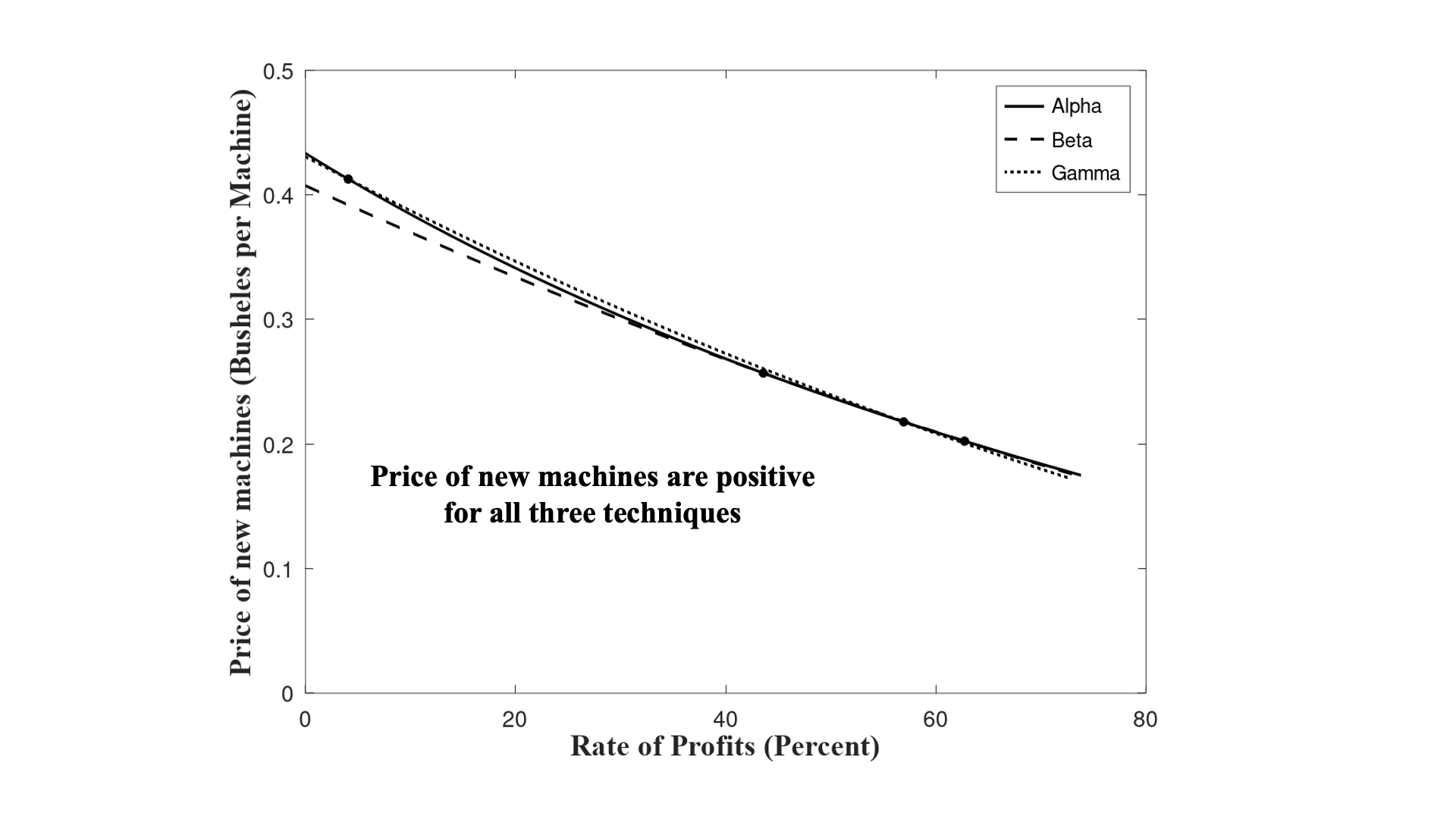
I can find when the price of each machine is positive. For new machines (Figure 2), their prices are positive:

• For Alpha, when 0 < r < 74.2 percent
• For Beta, when 0 < r < 73.8 percent
• For Gamma, when 0 < r < 72.7 percent.

The upper limits are approximate. The wage curves in Figure 1, at the top of this post, intersect the axis for the rate of profits at these upper limits.

Figure 2: Prices of New Machines

One-year old machines have positive prices (Figure 3):

• For Beta, when 43.6 percent < r < 62.7 percent
• For Gamma, when 4.1 percent < r < 56.9 percent

Under Alpha, the machine is discarded after one year, and the prices of old machines are identically zero. Beta is not operated outside the limits in which the price curve for Beta intersects the abscissa in Figure 3. If the machine were being truncated after two years, it would pay to discard it after one year. The same applies to Gamma. The analysis, so far, shows that Alpha would be adopted at the extremes of low and high rates of profits,

Figure 3: Prices of One-Year Old Machines

Two-year old machines have positive prices (Figure 4):

• For Gamma, when 0 < r < 55.7 percent

Since the price of a two year old machine is negative for rates of profits greater than at the switch point, Gamma will not be operated at those rates of profits.

Figure 4: Prices of Two-Year Old Machines

I can now summarize the analysis of the choice of technique for this example. Managers of firms will not adopt a technique when the outputs of a process in the technique has a negative price. Thus, each technique will be adopted in the following intervals:

• Alpha, for 0 < r < 4.1 percent and 62.7 percent < r < 74.2 percent
• Beta, for 55.7 percent < r < 62.7 percent
• Gamma, for 4.1 percent < r < 55.7 percent

Now, I can look at what happens around the three switch points:

• Around r = 62.7 percent, a lower interest rate is associated with a switch from Alpha to Beta, a more roundabout technique. But net output per worker falls. A more roundabout technique is less capital-intensive.
• Around r = 55.7 percent, a lower interest rate is associated with a switch from Beta to Gamma, a more roundabout technique. And net output per worker rises.
• Around r = 4.1 percent, a lower interest rate is associated with a switch from Gamma to Alpha, a less roundabout technique. And net output per worker rises. A less roundabout technique is more capital-intensive.

Only the middle switch point validates Austrian capital theory. Clearly, economists of the Austrian school have made mistakes in logic.

I like to note that the above argument is not about aggregation.

5.0 Conclusion

The above constitutes a proof that Austrian capital theory is mistaken. It relies on an identification, in the example, of more roundaboutness with a longer economic life of a machine. Austrian economists have tried to express their central insight that a greater use of capital is equivalent to a greater use of time in several disparate ways.

Perhaps greater roundaboutness should be identified with the use of different, better machines. By putting aside some time each day, Crusoe can make a net, instead of relying on whatever lies about at hand when catching fish. Or perhaps roundaboutness should be measured by a average period of production. Or by a financial measure of duration. What about those Hayekian triangles?

Since the central insight happens to be wrong, each of these formulations can be demonstrated to be, at best, ad hoc. But for each formulation, to be shown wrong in detail, requires a separate argument. Such can be provided and has been provided for most. Both Austrians and more mainstream marginalists have been in the position, for decades, that every economist is their own capital-theorist.

References

• Baldone, Salvatore (1974), Il capitale fisso nello schema teorico di Piero Sraffa, Studi Economici, XXIV(1): 45-106. Trans. in Pasinetti (1980).
• Kurz, Heinz D. and Neri Salvadori. 1995. Theory of Production: A Long-Period Analysis. Cambridge: Cambridge University Press.
• Pasinetti, Luigi L., (1980) (ed.), Essays on the Theory of Joint Production, New York: Columbia University Press

Three Examples For The Cambridge Capital Controversy

Figure 1: A Parameter Space

1.0 Introduction

I have been reconstructing some of my examples. The first example in this post is from here. I am thinking of writing a draft article, as mentioned here. While I am at it, I thought I would also work through the examples in Garegnani (1966) and Bruno, Burmeister & Sheshinski (1966), both from the symposium in the Quarterly Journal of Economics of that year.

2.0 The Emergence of the Reverse Substitution of Labor

This section presents an example with circulating capital alone. Table 1 presents the technology for an economy in which two commodities, iron and corn, are produced. Managers of firms know of one process for producing iron and two for producing corn. Each process is specified by coefficients of production, that is, the required physical inputs per unit output. The Alpha technique consists of the iron-producing process and the first corn-producing process. Similarly, the Beta technique consists of the iron-producing process and the second corn-producing process. At any time, managers of firms face a problem of the choice of technique

Table 1: Technology for the Reverse Substitution of Labor

Input	Industry
	Iron	Corn
		Alpha	Beta
Labor	a0,1=1	aα0,2=16/25	aβ0,2
Iron	a1,1=9/20	aα1,2=1/625	aβ1,2
Corn	a2,1=2	aα2,2=12/25	aβ2,2=27/400

Two parameters are not given numerical values in this specification of technology. The approach taken here is to examine a local perturbation of parameters in a two-dimensional slice of the higher dimensional parameter space defined by the coefficients of production in particular numeric examples. With wages paid out of the surplus product at the end of the period of production, the wage curves for the two techniques are depicted in Figure 2 for a particular parametrization of the coefficients of production. The Beta technique is cost-minimizing for any feasible distribution of income. If the wage is zero and the workers live on air, the Alpha technique is also cost-minimizing.

Figure 2: Wage Curves with Two Fluke Switch Point

A switch point is defined in this model of circulating capital to be an intersection of the wage curves. These switch points, for the particular parameter values illustrated in Figure 2, are fluke cases. Almost any variation in the model parameters destroys their interesting properties. A switch point exists at a rate of profits of -100 percent only along a knife edge in the parameter space (Figure 1). Likewise, a switch point exists on the axis for the rate of profits only along another knife edge. The illustrated example, with two fluke switch points, arises at a single point in the parameter space, where these two partitions intersect.

Figure 1 depicts a partition of the parameter space around the point with these two fluke switch points. Below the horizontal line, the switch point on the axis for the rate of profits has disappeared below the axis. The Beta technique is cost-minimizing for all feasible non-negative rates of profits. Above this locus, the Alpha technique is cost-minimizing for a low enough wage or a high enough feasible rate of profits.

In the northwest, the switch point at a negative rate of profits occurs at a rate of profits lower than 100 percent. Around the switch point at a positive rate of profits, a lower wage is associated with the adoption of the corn-producing process with a larger coefficient for labor. That is, at a higher wage, employment is lower per unit of gross output in the corn industry.

In the northeast of Figure 1, the switch point for a positive rate of profits exhibits the reverse substitution of labor. Around this switch point, a higher wage is associated with the adoption of a process producing the consumer good in which more labor is employed per unit of gross output. The other switch point exists for a rate of profits between -100 percent and zero. Steedman (2006) presents examples with this phenomenon in models with other structures

Qualitative changes in the wage frontier exist in the parameter space away from the part graphed in Figure 1. The analysis presented here is of local perturbations of the depicted fluke case.

2.0 Example from Garegnani (1966)

I think of Luigi Pasinetti as the first to show that David Levhari's non-(re)switching theorem is false. But the counter-example that he presented at the September 1965 Rome Congress of the Econometric Society did not quite meet all of the assumptions of Levhari's theorem.

Table 2 defines the coefficients of production for the counter-example from Pierangelo Garegnani's paper in the QJE symposium devoted to the topic. Figure 3 presents the wage curves for the example. Switch points are at 10 percent and 20 percent, appealingly reasonably small rates of profits. But the wage curves are visually hard to distinguish. The switch points are more apparent in the plot of extra profits at Alpha prices, in the right pane.

Table 2: Technology for a Reswitching Example

Input	Industry
	Iron	Corn
		Alpha	Beta
Labor	a0,1=89/10	aα0,2=9/50	aβ0,2=3/2
Iron	a1,1=0	aα1,2=1/2	aβ1,2=1/4
Corn	a2,1=379/423	aα2,2=1/10	aβ2,2=5/12

Figure 3: Wage Curves for a Reswitching Example

In some sense, it is unfair to criticize scholars of that time for not creating more apparent examples. The tools I have are much more advanced for seeing the effect of perturbing a coefficient. And, nevertheless, I still have some examples that are hard to see the 'perverse' results.

3.0 Example from Bruno, Burmeister & Sheshinski (1966)

The counter example from Michael Bruno, Edwin Burmeister, and Eytan Sheshinski's paper in the QJE symposium has more a visually striking wage frontier. Table 3 presents the coefficients of production. (I have reordered the industries.) Figure 4 plots the wage curves. The switch points are at approximately 46.58 percent and 166.88 percent or wages of approximately 0.8065 and 0.2595 bushels per person-year.

Table 3: Technology for Another Reswitching Example

Input	Industry
	Iron	Corn
		Alpha	Beta
Labor	a0,1=1	aα0,2=33/100	aβ0,2=1/100
Iron	a1,1=0	aα1,2=1/50	aβ1,2=71/100
Corn	a2,1=1/10	aα2,2=3/10	aβ2,2=0

Figure 4: Wage Curves for another Reswitching Example

Many like to quote Paul Samuelson declaration that:

"...the simple tale told by Jevons, Böhm-Bawerk, Wicksell, and other neoclassical writers - alleging that, as interest rate falls in consequence of abstention from present consumption in favor of future, technology must become in some sense more 'roundabout,' more 'mechanized,' and more 'productive' - cannot be universally valid." -- Paul A. Samuelson (1966).

Bruno, Burmeister & Sheshinski are just as clear:

"Numerical examples and the realization that switching points are roots of n-th degree polynomials (and therefore numerous) have convinced us that reswitching may well occur in a general capital model." - Bruno, Burmeister & Sheshinski (1966, p. 527)

Somehow, empirical work has not made it apparent all of these possible real roots, despite the exploration of economies with many industries. I like this quotation too:

"Although the latter sufficiency condition is again highly restrictive, it may be somewhat less restrictive than the former one: note the latter allows changes of single activities while the former does not. We might also observe that the latter condition seems to be the most natural extension of our previous two-sector nonswitching theorem... Let us again stress that, except for highly exceptional circumstances, techniques cannot be ranked in order of capital intensity. We thus conclude that reswitching is, at least theoretically; a perfectly acceptable case in the discrete capital model." - Bruno, Burmeister & Sheshinski (1966, p. 545)

I skimmed the sufficiency condition. I think technologies with different capital goods used in different techniques are ruled out. Likewise, processes in the same industry in which some capital goods are increased and others are decreased might also be ruled out. It is the general case that technology can be such that reswitching is possible.

Variations In Switch Points With Markups In The 'Corn' Industry

Figure 1: Variation of Switch Points with the Markup in the Corn Industry

1.0 Introduction

I have been re-creating some of my past analyses. The graphs in this post look a bit different because I impose a requirement that the relative markups sum to unity.

2.0 Technology

Consider an economy which produces three commodities, iron, steel, and corn, with the technology specified in Table 1. Two processes are available for producing each commodity. The coefficients of production in a column specify the person-years of labor, tons of iron, tons of steel, and bushels of corn required to produce a unit of output of the given industry.

Table 1: The Technology

Input	Iron Industry		Steel Industry		Corn Industry
	a	b	c	d	e	f
Labor	1/3	1/10	5/2	7/20	1	3/2
Iron	1/6	2/5	1/200	1/100	1	0
Steel	1/200	1/400	1/4	3/10	0	1/4
Corn	1/300	1/300	1/300	0	0	0

Eight techniques (Table 2) are defined for this technology. Each technique is defined by the operation of one process in each of the three industries. All three commodities are Sraffian basics in all techniques. That is, each commodity is a direct or indirect input in the production of all commodities. For example, iron is used directly as an input in the first corn-producing process, and steel is used indirectly in producing corn with this process since steel is an input in either iron-producing process

Table 2: Techniques

Technique	Processes
Alpha	a, c, e
Beta	a, c, f
Gamma	a, d, e
Delta	a, d, f
Epsilon	b, c, e
Zeta	b, c, f
Eta	b, d, e
Theta	b, d, f

3.0 Prices of Production

Prices of production are defined here for given ratios of markups among industries. The ratios of rates of profits among industries are assumed stable, but rates of profits are not necessarily uniform. Lack of uniformity in rates of profits can result from variations in evaluations of profits among industries due to idiosyncratic properties of investment; from barriers to entry arising from, for example, secrets in manufacture; and from legal monopolies (D’Agata 2018). Let s₁ r, s₃ r, and s₃ r be the rate of profits in the iron, steel, and corn industries respectively. I call r the scale factor for the rate of profits. The usual system of equations, with labor advanced, must be satisfied for prices of production for a given technique.

As a matter of scaling, suppose the markups lie on a simplex:

s₁ + s₂ + s₃ = 1

Suppose that a bushel of corn is the numeraire. In drawing various graphs, I consider only variations in the markup in the corn industry, with markups in producing iron and steel assumed identical:

s₁ = s₂

The solution to this system, for each technique, has a single degree of freedom, which can be expressed with the wage as a function of the scale factor for the rate of profits

4.0 The Choice of Technique with Competitive Markets

Figure 1 graphs the wage curves for four techniques, given competitive markets. The same relative markups are obtained in all industries. The cost-minimizing technique at a given wage maximizes the scale factor for the rate of profits. The cost-minimizing technique at a given scale factor maximizes the wage. The outer frontier of all wage curves shows the variation of the cost-minimizing technique with distribution. Wage curves are graphed in Figure 1 only for the techniques on the outer frontier. This type of figure, usually for competitive markets, is the most well-known graph in post-Sraffian price theory

Figure 2: Capital-Reversing with Competitive Markets

Around the so-called perverse switch point, the firms in the corn industry switch from the second corn-producing process to the first at a lower wage. That is, they adopt a process that requires less labor to be hired per bushel of corn produced gross. This is known as the reverse substitution of labor (Han and Schefold 2006). For the economy as a whole, the technique adopted at a lower wage requires less labor per unit of net output. This is a consequence of capital-reversing as manifested in a comparison of stationary states (Harris 1973).

5.0 Fluke Cases

Five fluke cases can be found by perturbing the relative markup in the corn industry (Table 3). Figure 3 depicts the wage frontier for the first fluke case. This markup occurs when reswitching is just emerging.

Table 3: Fluke Switch Points

Markup for Corn	Fluke Case
s3 ≈ 0.211996	Reswitching pattern for Gamma vs. Delta.
s3 ≈ 0.249246	Four technique pattern for Gamma, Delta, Eta, and Theta.
s3 ≈ 0.8232415	Alpha vs Beta switch point at wage of zero.
s3 ≈ 0.8696757	Four technique pattern for Alpha, Beta, Gamma, and Delta.
s3 ≈ 0.9307414	Beta vs Delta pattern over r axis

Figure 3: Wage Curves for Gamma and Delta Tangent at Switch Point

6.0 The Choice of Technique with the Full Range of the Markup in the Corn Industry

Figure 1, at the top of this post, is my new type of diagram illustrated for depicting the analysis of the choice of technique. The abscissa is the markup in the corn industry, with given markups of unity in the iron and steel industry. The maximum wage and the wage at switch points along the frontier are plotted. The number and sequence of switch points along the wage frontier are invariant in each numbered region. Fluke switch points partition the numbered regions. Figure 4 enlarges Figure 1 on the right for low wages

Figure 4: Variation of Switch Points with the Markup (Detail)

The qualitative properties of the wage frontier are invariant in each numbered region in Figures 1 and 4. Table 4 describes each numbered region. The cost-minimizing technique along the wage frontier is listed, from a wage of zero to the maximum wage. Some salient properties of switch points and the cost-minimizing technique are summarized in Table 5. Figure 2 depicts the wage frontier for a markup in the corn-industry in region 3, while Figure 3 depicts the wage frontier on the boundary between regions 1 and 2.

Table 4: Variations in the Cost-Minimizing Technique

Region	Range	Technique
1	0 ≤ w ≤ w1	Alpha
	w1 ≤ w ≤ w2	Gamma
	w2 ≤ w ≤ wmax,η	Eta
2	0 ≤ w ≤ w1	Alpha
	w1 ≤ w ≤ w2	Gamma
	w2 ≤ w ≤ w3	Delta
	w3 ≤ w ≤ w4	Gamma
	w4 ≤ w ≤ wmax,η	Eta
3	0 ≤ w ≤ w1	Alpha
	w1 ≤ w ≤ w2	Gamma
	w2 ≤ w ≤ w3	Delta
	w3 ≤ w ≤ w4	Theta
	w4 ≤ w ≤ wmax,η	Eta
4	0 ≤ w ≤ w1	Beta
	w1 ≤ w ≤ w2	Alpha
	w2 ≤ w ≤ w3	Gamma
	w3 ≤ w ≤ w4	Delta
	w4 ≤ w ≤ w5	Theta
	w5 ≤ w ≤ wmax,η	Eta
5	0 ≤ w ≤ w1	Beta
	w1 ≤ w ≤ w2	Delta
	w2 ≤ w ≤ w3	Theta
	w3 ≤ w ≤ wmax,η	Eta
6	0 ≤ w ≤ w1	Delta
	w1 ≤ w ≤ w2	Theta
	w2 ≤ w ≤ wmax,η	Eta

Table 5: Notes on Regions

Region	Summary
1	No reswitching, no capital-reversing, no reverse substitution of labor, no process recurrence.
2	Reswitching of techniques between Gamma and Delta. Capital-reversing and the reverse substitution of labor at the switch point between Gamma and Delta at the lower wage. Process recurrence of the first process in the corn industry.
3	No reswitching. Capital-reversing and the reverse substitution of labor at the switch point between Gamma and Delta. Process recurrence of the first process in the corn industry.
4	No reswitching. Capital-reversing and the reverse substitution of labor at the switch point between Gamma and Delta. Process recurrence of both processes in the corn industry.
5	No reswitching, no capital-reversing, no reverse substitution of labor, no process recurrence.
6	No reswitching, no capital-reversing, no reverse substitution of labor, no process recurrence.

This example allows for a graphical display showing that reswitching arises with an increased markup in corn-production, starting from a markup much less than in other industries. The ‘perverse’ switch point between Gamma and Delta remains on the wage frontier after the other switch point between these techniques falls off the frontier at a higher markup. Eventually, the ‘perverse’ switch point is no longer on the frontier when corn-production has a much higher markup than other industries.

7.0 Conclusion

The properties of the wage frontier might be thought to have some impact on the struggle between capitalists and workers. These properties can be altered both by technical change and by variations in relative market power among capitalists.