Structural Economic Dynamics And Reswitching In A One-Good Model

This post, as suggested, extends this one-good example. I assume a constant returns-to-scale technology, as specified in Tables 1 and 2. Labor is advanced to the capitalists, and wages are paid out of the surplus at the end of the year (period of production). The capitalists (incorrectly) expect the technology in existence at the start of the year to continue to exist. I assume prices of (re)production prevail.

Table 1: Inputs for The Technology

Input	Process
	(I)	(II)	(III)
Labor	30 eσ0,1(1 - t)	180 eσ0,2(1 - t)	(39/2) eσ0,3(1 - t)
New Widgets	1	0	0
One-Year Old Widgets	0	1	0
Two-Year Old Widgets	0	0	1

Table 2: Outputs for The Technology

Output	Process
	(I)	(II)	(III)
New Widgets	3 eσ1,1(t - 1)	(7/4) eσ1,2(t - 1)	(237/20) eσ1,3(t - 1)
One-Year Old Widgets	1	0	0
Two-Year Old Widgets	0	1	0

Only a newly produced widget is a consumer good. Old widgets can be used in production for two more years. The economic lifetime of a widget (machine) may be less than its physical life. Free disposal is assumed. I define techniques:

• Alpha: The widget is discarded after one year.
• Beta: The widget is discarded after two years.
• Gamma: The widget is discarded after three years.

The specification of technology allows for productivity to increase in each process, both because labor is saved and because more output is produced with a unit input of widgets. Figure 1 shows one of my pattern diagrams, in which the specification of increased productivity results from reducing the parameter space to three dimensions.

I identify two of my patterns in this diagram, a pattern over the wage axis and a reswitching pattern. In Region 2, reswitching occurs. Around the switch point at the lower rate of profits, a higher rate of profits is associated with a truncation of the economic life of a machine to one years. This logical possibility contradicts Austrian capital theory, in which a scarcity of capital results in a higher rate of profits and a longer period of production. In circulating capital models, the switch point at the lowest rate of profits is 'non-perverse', unlike here. I thing Ian Steedman made the same observation decades ago.

Structural Economic Dynamics with a Choice of Technique in General

Many - not all - of my recent numerical examples have a certain abstract pattern:

1. At the start of the time under consideration, one technique is uniquely cost minimizing, for all feasible rates of profits.
2. Coefficients of production decline or some markups over the normal rate of profits vary.
3. A fluke switch point appears.
4. Switch points move along the wage frontier, and interesting phenomena occur. These can be other fluke switch points. Reswitching, the recurrence of techniques, capital-reversing, the reverse substitution of labor, or process recurrence might arise for some time.
5. Eventually, these interesting phenomena disappear, and another technique is uniquely cost minimizing, for all feasible rates of profits.

I have not been looking at random technology. The occurrence of a fluke switch point is not surprising in my examples. Neither is some of the phenomena mentioned in (4). I have been deliberately creating examples to highlight some of these possibilities. But I have often found a second or more fluke switch points arising that I did not expect. I have also created examples in which one technique gets replaced with another, but in which reswitching, etc. do not occur.

My program remains unfinished. In these posts and papers, I have suggested the possibilities of some proofs and additional fluke switch points. I have yet to even begin considering how the changes in the wage frontier I have been investigating might manifest themselves in the movement of market prices. I could do more with markups varying among industry. I have yet to provide examples with land and fixed capital, where the wage frontier is not the appropriate tool for analyzing the choice of technique.

Update To A Start On A Catalog Of Switch Point Patterns Of High Co-Dimension

I have been looking at patterns of switch points. A pattern is a configuration of switch points helpful for perturbation analysis for the choice of technique. I am curious how the switch points and the wage curves along the wage frontier can alter with parameters, in a model of the production of commodities. Such a parameter can be a coefficient of production; time, where a number of parameters are functions of time; or the markup in an industry or a number of industries. A normal form exists for each pattern. The normal form describes how the techniques and switch points along the frontier vary with a selected parameter value. Each pattern is defined by the equality of wage curves at a switch point and one or more additional conditions. The co-dimension of a pattern is the number of additional conditions.

I claim that local patterns of co-dimension one, with a switch point at a non-negative, feasible rate of profits can be described by four normal forms. I have defined these patterns as a pattern over the axis for the rate of profits, a pattern across the wage axis, a three-technique pattern, and a reswitching pattern. This post is an update, and continues to examine global patterns, local patterns with a co-dimension higher than unity, and sequences of local patterns. Some examples are:

• A switch point that is simultaneously a pattern across the wage axis and a reswitching pattern (a case of a real Wicksell effect of zero). This illustrates a pattern of co-dimension two.
• A reswitching example with one switch point being a pattern across the wage axis (another case of a real Wicksell effect of zero). This is a global pattern.
• An example with a pattern across the wage axis and a pattern over the axis for the rate of profits. This is a global pattern.
• A pattern like the above, but with both switch points being defined by intersections of wage curves for the same two techniques. This is a global pattern.
• Two switch points, with both being reswitching patterns, can be found from a partition of a parameter space where two loci for reswitching patterns intersect. This gestures towards a global pattern.
• A pattern across the point where the rate of profits is negative one hundred percent, combined with a switch point, for the same techniques, with a positive rate of profits (of interest for the reverse substitution of labor). This is a global pattern.
• An example where every point on the frontier is a switch point. This is a global pattern of an uncountably infinite co-dimension.
• Speculation on three sequences of patterns of co-dimension one that result in one technique replacing another, in an intermediate range of the rate of profits, along the wage frontier.
• A switch point for a four-technique pattern (due to Salvadori and Steedman). This is a local pattern of co-dimension two.
• Further analysis of the above example.
• An example of a four-technique pattern in a model with three produced commodities. This local pattern of co-dimension two results in one technique replacing another, in an intermediate range of the rate of profits, along the wage frontier.
• Further analysis of the above example. Two normal forms are identified for four-technique patterns.

The above list is not complete. More types of fluke switch points exist. Some, like the examples of a real Wicksell effect of zero, I thought, should be of interest for themselves to economists. Others show examples of parameters where the appearance of the wage frontier, at least, changes with perturbations of the parameters. I have used these patterns to tell stories about how technical change or a change in markups (that is, structural economic dynamics) can result in reswitching, capital reversing, or the reverse substitution of labor appearing on or disappearing from the wage frontier.

I would like to see that in at least some cases, short run dynamics changes qualitatively with such perturbations. But this seems to be beyond my capabilities.

Start of a Catalogue of Flukes of Fluke Switch Points

I claim that the pattern analysis I have defined can be used to generate additional fluke switch points. I am particularly interested in switch points that are flukes in more than one way (local patterns of co-dimension higher than one) and fluke switch points that are combined with other fluke switch points or some aspect of other switch points (global patterns). I have already generated some examples, not always with pattern analysis.

• Fluke switch points of higher co-dimension
• A switch point that is simultaneously a pattern across the wage axis and a reswitching pattern (a case of a real Wicksell effect of zero).
• A switch point combining four three-technique patterns (due to Salvadori and Steedman).
• Fluke switch points combined with other switch points
• A reswitching example with one switch point being a pattern across the wage axis (another case of a real Wicksell effect of zero).
• An example with a pattern across the wage axis and a pattern over the axis for the rate of profits.
• Two switch points with both being reswitching patterns can be found from a partition of a parameter space where two loci for reswitching patterns intersect.
• A pattern across the point where the rate of profits is negative one hundred percent, combined with a switch point, for the same techniques, with a positive rate of profits (of interest for the reverse substitution of labor).
• An example where every point on the frontier is a switch point.

The above list is not complete. More types of fluke switch points exist. Some, like the examples of a real Wicksell effect of zero, I thought, should be of interest for themselves to economists. Others show examples of parameters where the appearance of the wage frontier, at least, changes with perturbations of the parameters. I would like to see that in at least some cases, short run dynamics changes qualitatively with such perturbations. But this seems to be beyond my capabilities.

Maybe I'll update this post some day, if I create more examples.

Bifurcation Analysis of a Two-Commodity, Three-Technique Technology

Figure 1: A Bifurcation Diagram

This post expands on this previous post. The technology is the same, but the rates of decrease of the coefficients of production in the Beta and Gamma corn-producing processes are not fixed. Instead, I consider the full range of parameter values. (I find the graphs produced by bifurcation analysis interesting for this case, but I think a two-commodity example can be found with more pleasing diagrams.)

Anyways, Figure 1 shows a bifurcation diagram for the parameter space in this example. The region numbered 8 is not visible on the graph. Accordingly, Figure 2 below shows a much expanded picture of the parameter space around that region. The specific parameter values in the previous post lead to a temporal path along the dashed ray extending from the origin in Figure 1. (The numbering of regions in this post and the previous post do not correspond.) Although it is not obvious, the locus of points bifucating regions 9 and 10 eventually, somewhere to the right of the region shown in Figure 1 eventually decreases in slope and intercepts the dashed ray.

Figure 2: Blowup of a Part of the Bifurcation Diagram

As usual, each numbered region corresponds to a definite sequence of cost-minimizing techniques contributing wage curves along the wage frontier. Table 1 lists this sequence for each region. Some notes on switch points are provided. A switch point is called "normal" merely if it conforms to outdated neoclassical intuition. In other words, such a switch point exhibits negative real Wicksell effects. In the example, regions also exist where switch points exhibit positive real Wicksell effects.

Table 1: Cost-Minimizing Techniques by Region

Region	Cost-Minimizing Techniques	Notes
1	Alpha	One technique cost-minimizing.
2	Alpha, Beta	"Normal" switch point.
3	Beta, Alpha, Beta	Reswitching. Switch pt. at highest r is "perverse".
4	Beta	One technique cost-minimizing.
5	Alpha, Gamma	"Normal" switch point.
6	Alpha, Gamma, Beta	"Normal" switch points.
7	Beta, Alpha, Gamma, Beta	Recurrence of techniques. Switch pt. at highest r is "perverse".
8	Beta, Alpha, Beta, Gamma, Beta	Two reswitchings, two "perverse" switch pts.
9	Gamma	One technique cost-minimizing.
10	Gamma, Beta	"Normal" switch point.
11	Beta, Gamma, Beta	Reswitching. Switch pt. at highest r is "perverse".

One can compare and contrast the above bifurcation diagram with the one in this post. The latter bifurcation diagram is for a specific instance of the Samuelson-Garegnani model, in which the basic commodity varies among techniques. (I have a more recent write-up of that bifurcation analysis linked to here.)

Reswitching Without a Reswitching Bifurcation

Figure 1: A Bifurcation Diagram

This post presents another example of bifurcation analysis applied to structural economic dynamics with a choice of technique. This example illustrates:

• Two reswitching examples appear and disappear without a reswitching bifurcation ever occurring, at least on the wage frontier.
• Two bifurcations over the wage axis arise. At the time each bifurcation of this type occurs, another switch point for the same techniques exhibits a real Wicksell effect of zero. Thus, for each, a switch point transitions from being a "normal" switch point to a "perverse" one exhibiting capital-reversing.
• Each of the four types of bifurcations of co-dimension one that I have identified have no preferred temporal order. For example, a bifurcation over the wage axis can add a switch point to the wage frontier. And another such bifurcation can remove a switch point, as time advances.
• The maximum rate of profits approaches an asymptote from below as time increase without bound.

Table 1 specifies the technology for this example, in terms of two parameters, σ and φ. Managers of firms know of one process for producing iron and of three processes for producing corn. Each process is defined in terms of coefficients of production, which specify the quantities of labor, iron, and corn needed to produce a unit output for that process. All processes exhibit constant returns to scale; require a year to complete; and totally use up, in producing their output, the capital goods required as input. I consider the special case in which the rate of decrease of the coefficients of production in the Beta corn-producing process, σ, is 5 percent, and the rate of decrease of coefficients in the Gamma corn-producing process, φ, is 10 percent.

Table 1: Processes For Producing Iron and Corn

Input	Iron Industry	Corn Industry
		Alpha	Beta	Gamma
Labor	1	0.89965	0.71733 e-σ t	1.28237 e-φ t
Iron	0.45	0.025	0.00176 e-σ t	0.03375 e-φ t
Corn	2	0.1	0.53858 e-σ t	0.13499 e-φ t

Three techniques are available for producing a net output of, say, corn, while reproducing the capital goods used as input. The Alpha process consists of the iron-producing process and the corn-producing process labeled Alpha. And so on for the Beta and Gamma techniques.

The choice of technique is analyzed in the usual way. I assume that labor is advanced, and wages are paid out of the surplus product at the end of the year. Corn is taken as numeraire. A wage curve can be drawn for each technique, given the coefficients of production prevailing at a given moment in time. Figure 1 illustrates a case of the recurrence of techniques in the example. The cost-minimizing technique is found by constructing the outer frontier of the wage curves. In Figure 2, the cost-minimizing techniques are Beta, Alpha, Gamma, and Beta, in that order. The switch point at approximately 57 percent exhibits capital-reversing. Around the switch point, a higher wage is associated with the adoption of a more labor-intensive technique. If prices of production prevail, firms will find it cost-minimizing to hire more workers at a higher wage, given net output.

Figure 2: Wage Curves in Region 4

Figure 3 illustrates the analysis of the choice of technique for all time. Switch points along the frontier and the maximum rate of profits are plotted versus time. Figure 1, at the top of this post, is a blowup of Figure 3 from time zero to a time of five years. These pictures show which technique is cost-minimizing at each rate of profits, at each moment in time. Bifurcations are also shown. Table 2 lists the cost-minimizing techniques in each region between the bifurcations.

Figure 3: An Extended Bifurcation Diagram

Table 2: Cost-Minimizing Techniques by Region

Region	Cost-Minimizing Techniques	Notes
1	Alpha	One technique cost-minimizing.
2	Alpha, Beta	"Normal" switch point.
3	Beta, Alpha, Beta	Reswitching. Switch pt. at highest r is "perverse".
4	Beta, Alpha, Gamma, Beta	Recurrence of techniques. Switch pt. at highest r is "perverse".
5	Beta, Gamma, Beta	Reswitching. Switch pt. at highest r is "perverse".
6	Gamma, Beta	"Normal" switch point.
7	Gamma	One technique cost-minimizing. Maximum r approaches an asymptote.

I suppose I can extend this example to partition the complete parameter space, as in this example, with an updated write-up here. That analysis will demonstrate, by example, that this sort of bifurcation analysis applies to cases in which multiple commodities are basic in multiple techniques. It is not confined to the special case of the Samuelson-Garegnani model. I am also thinking that I could perform a bifurcation analysis where parameters that vary include the ratio of the rates of profits in various industries, as in these examples of a model of oligopoly. Maybe such an analysis will yield an empirically relevant tale of the evolution of economic duality (also known as segmented markets).

Bifurcation Analysis Applied to Structural Economic Dynamics with a Choice of Technique

Variation of Switch Points with Technical Progress in Two Industries

I have a new working paper - basically an update of one I have previously described.

Abstract: This article illustrates the application of bifurcation analysis to structural economic dynamics with a choice of technique. A numerical example of the Samuelson-Garegnani model is presented in which technical progress is introduced. Examples of temporal paths through the parameter space illustrate variations of the wage frontier. A single technique is initially uniquely cost-minimizing for all feasible rates of profits. Eventually, the technique for which coefficients of production decrease at the fastest rate is always cost-minimizing. This example illustrates possible variations in the existence of Sraffa effects, which arise during the transition between these positions.

Structural Economic Dynamics with a Choice of Technique: A Numerical Example

A Bifurcation Diagram with Two Temporal Paths

I have a working paper with the post title. Here's the abstract:

This article illustrates the application of bifurcation analysis to structural economic dynamics with a choice of technique. A numerical example of the Samuelson-Garegnani model is presented in which technical change is introduced. Examples of temporal paths through the parameter space illustrate variations of the wage frontier. A single technique is initially uniquely cost-minimizing for all feasible rates of profits. Eventually, the technique for which coefficients of production decrease at the fastest rates is always cost-minimizing. During the transition between these positions, reswitching, the recurrence of techniques, and capital-reversing can arise. This example emphasizes the importance of fluke switch points and illustrates possible variations in the existence of Sraffa effects.

Generic Bifurcations and Switch Points

This post states a mathematical conjecture.

Consider a model of prices of production in which a choice of technique exists. The parameters of model consist of coefficients of production for each technique and given ratios for the rates of profits among industries. The choice of technique can be analyzed based on wage curves. A point that lies simultaneously on the outer envelope of all wage curves and the wage curves for two techniques (for non-negative wages and rates of profits not exceeding the maximum rates of profits for both techniques) is a switch point.

Conjecture: The number of switch points is a function of the parameters of the model. The number of switch points varies with variations in the parameters.

• A pair of switch points can arise if:
• One wage curve dominates another for one set of parameter values.
• The wage curves become tangent at a single switch point, for a change in one parameter.
• The point of tangency breaks up into two switch points (reswitching) as that parameter continues in the same direction.
• A switch point can disappear (for an economically relevant ranges of wages) if:
• A switch point exists for some set of parameter values.
• For some variation of a parameter, that switch point becomes the intersection of both wage curves with one of the axes (the wage or the rate of profits).
• A further variation of the parameter in the same direction leads to the point of intersection of the wage curves falling out of the first quadrant.
• Like the above, but a switch point can disappear if a variation in a parameter results in that intersection of two wage curves falling off the outer envelope. (A third wage curve becomes dominant for the wage at which the intersection occurs.)

The above three possibilities are the only generic bifurcations in which the number of switch points can change with model parameters.

Proof: By incredibility. How could it be otherwise?

I claim that the above conjecture applies to a model with n commodities, not just the two-commodity example I have previously analyzed. It applies to a choice among as many finite techniques as you please. Different techniques may require different capital goods as inputs. Not all commodities need be basic.

In actuality, I do not know how to prove this. I am not sure what it means for a bifurcation to be generic in the above conjecture, but I want to allow for a combination of, say, two of the three possibilities. For example, the point of tangency for two wage curves (in the first case) may simultaneously be the intersection of both wage curves with the axis for the rate of profits. In this case, only one switch point arises with continuous variation of model parameters; the other falls below the axis for the rate of profits. I want to say such a bifurcation is non-generic, in some sense.

This post needs pictures. I assume the third possibility can arise for some parameter in at least one of these examples. (Maybe I need to think harder to be sure that the number of switch points changes. What do I want to say is non-generic here?) I have an example in which a switch point disappears by falling below the axis for the rate of profits, but I do not have an example of a switch point disappearing by crossing the wage axis.

Bifurcations And Switchpoints

I have organized a series of my posts together into a working paper, titled Bifurcations and Switch Points. Here is the abstract:

This article analyzes structural instabilities, in a model of prices of production, associated with variations in coefficients of production, in industrial organization, and in the steady-state rate of growth. Numerical examples are provided, with illustrations, demonstrating that technological improvements or the creation of differential rates of profits can create a reswitching example. Variations in the rate of growth can change a "perverse" switch point into a normal one or vice versa. These results seem to have implications for the stability of short-period dynamics and suggest an approach to sensitivity analysis for certain empirical results regarding the presence of Sraffa effects.

Here are links to previous expositions of parts of this analysis:

• Variation in selected coefficients of production:
• Variation of switch points
• A bifurcation diagram
• A model of prices of production under oligopoly:
• The model
• Variation of switch points with markups
• A bifurcation diagram
• Bifurcations with variations in the rate of growth

In comments, Sturai suggests additional research with the model of oligopoly. One could take the standard commodity as such that it has no markup. What I am calling the scale factor for the rate of profits would be the rate of profits made in the production of the standard commodity. Markups for individual industries would be based on this. I have identified a problem, much like the transformation problem, in comparing and contrasting free competition and oligopoly. I would have to think about this.

Bifurcation Analysis in a Model of Oligopoly

Figure 1: Bifurcation Diagram

I have presented a model of prices of production in which the the rate of profits differs among industries. Such persistent differential rates of profits may be maintained because of perceptions by investors of different levels of risk among industries. Or they may reflect the ability of firms to maintain barriers to entry in different industries. In the latter case, the model is one of oligopoly.

This post is based on a specific numeric example for technology, namely, this one, in which labor and two commodities are used in the production of the same commodities. I am not going to reset out the model here. But I want to be able to refer to some notation. Managers know of two processes for producing iron and one process for producing corn. Each process is specified by three coefficients of production. Hence, nine parameters specify the technology, and there is a choice between two techniques. In the model:

• The rate of profits in the iron industry is rs₁.
• The rate of profits in the corn industry is rs₂.

I call r the scale factor for the rates of profits. s₁ is the markup for the rate rate of profits in the iron industry. And s₂ is the markup for the rate of profits in the corn industry. So, with the two markups for the rates of profits, 11 parameters specify the model.

I suppose one could look at work by Edith Penrose, Michal Kalecki, Joseh Steindl, Paolo Sylos Labini, Alfred Eichner, or Robin Marris for a more concrete understanding of markups.

Anyways, a wage curve is associated with each technique. And that wage curve results in the wage being specified, in the system of equations for prices of production, given an exogenous specification of the scale factor for the rates of profits. Alternatively, the scale factor can be found, given the wage. Points in common (intersections) on the wage curves for the two techniques are switch points.

Depending on parameter values for the markups on the rates of profits, the example can have no, one, or two switch points. In the last case, the model is one of the reswitching of techniques.

A bifurcation diagram partitions the parameter space into regions where the model solutions, throughout a region, are topologically equivalent, in some sense. Theoretically, a bifurcation diagram for the example should be drawn in an eleven-dimensional space. I, however, take the technology as given and only vary the markups. Figure 1, is the resulting bifurcation diagram.

The model exhibits a certain invariance, manifested in the bifurcation diagram by the straight lines through the origin. Suppose each markup for the rates of profits were, say, doubled. Then, if the scale factor for the rates of profits were halved, the rates of profits in each industry would be unchanged. The wage and prices of production would also be unchanged.

So only the ratio between the markups matter for the model solution. In some sense, the two parameters for the markups can be reduced to one, the ratio between the rates of profits in the two industries. And this ratio is constant for each straight line in the bifurcation diagram. The reciprocal of the slopes of the lines labeled 2 and 4 in Figure 1 are approximately 0.392 and 0.938, respectively. These values are marked along the abscissa in the figure at the top of this post.

In the bifurcation diagram in Figure 1, I have numbered the regions and the loci constituting the boundaries between them. In a bifurcation diagram, one would like to know what a typical solution looks like in each region and how bifurcations occur. The point in this example is to understand changes in the relationships between the wage curves for the two techniques. And the wage curves for the techniques for the numbered regions and lines in Figure 1 look like (are topologically equivalent to) the corresponding numbered graphs in Figure 2 in this post

The model of oligopoly being analyzed here is open, insofar as the determinants of the functional distribution of income, of stable relative rates of profits among industries, and of the long run rate of growth have not been specified. Only comparisons of long run positions are referred to in talking about variations, in the solution to a model of prices of production, with variations in model parameters. That is, no claims are being made about transitions to long period equilibria. Nevertheless, the implications of the results in this paper for short period models, whether ones of classical gravitational processes, cross dual dynamics, intertemporal equilibria, or temporary equilibria, are well worth thinking about.

Mainstream economists frequently produce more complicated models, with conjectural variations, or game theory, or whatever, of firms operating in non-competitive markets. And they seem to think that models of competitive markets are more intuitive, with simple supply and demand properties and certain desirable properties. I think the Cambridge Capital Controversy raised fatal objections to this view long ago. Reswitching and capital reversing show that equilibrium prices are not scarcity indices, and the logic of comparisons of equilibrium positions, in competitive conditions does not conform to the principle of substitution. In the model of prices of production discussed here, there is a certain continuity between imperfections in competition and the case of free competition. The kind of dichotomy that I understand to exist in mainstream microeconomics just doesn't exist here.

Continued Bifurcation Analysis of a Reswitching Example

Figure 1: Bifurcation Diagram

This post is a continuation of the analysis in this reswitching example. That post presents an example of reswitching in a model of the production of commodities by means of commodities. The example is one of an economy in which two commodities, iron and corn, are produced. Managers of firms know of two processes for producing iron and one process for producing corn. The definition of technology results in a choice between two techniques of production.

The two-commodity model analyzed here is specified by nine parameters. Theoretically, a bifurcation diagram should be drawn in nine dimensions. But, being limited by the dimensions of the screen, I select two parameters. I take the inputs per unit output in the two processes for producing iron as given constants. I also take as given the amount of (seed) corn needed to produce a unit output of corn, in the one process known for producing corn. So the dimensions of my bifurcation diagram are the amount of labor required to produce a bushel corn and the amount of iron input required to produce a bushel corn. Both of these parameters must be non-negative.

I am interested in wage curves and, in particular, how many intersections they have. Figure 1, above, partitions the parameter space based on this rationale. I had to think some time about what this diagram implies for wage curves. In generating the points to interpolate, my Matlab/Octave code generated many graphs analogous to those in the linked post. I also generated Figure 2, which illustrates configurations of wage curves and switch points, for the number regions and loci in Figure 1. So I had some visualization help, from my code, in thinking about these implications. Anyways, I hope you can see that, from perturbations of one example, one can generate an infinite number of reswitching examples.

Figure 2: Some Wage Curves

One can think of prices of production as (not necessarily stable) fixed points of short period dynamic processes. Economists have developed a number of dynamic processes with such fixed points. But I leave my analysis open to a choice of whatever dynamic process you like. In some sense, I am applying bifurcation analysis to the solution(s) of a system of algebraic equations. The closest analogue I know of in the literature is Rosser (1983), which is, more or less, a chapter in his well-known book.

Update (22 Jun 2017): Added Figure 2, associated changes to Figure 1, and text.

References

• J. Barkley Rosser (1983). Reswitching as a Cusp Catastrophe. Journal of Economic Theory V. 31: pp. 182-193.

Bifurcations With Variations In The Rate Of Growth

Figure 1: Perversity and Non-Perversity in the Labor Market Varying with the Rate of Growth

1.0 Introduction

I have been considering how the existence and properties of switch points vary with parameters specifying numerical examples of models of the production of commodities by means of commodities. Here are some examples of such analyses of structural stability. This post adds to this series.

I consider a change in sign of real Wicksell effects to be a bifurcation. In the model in this post, the steady state rate of growth is an exogenous parameter. So a change of sign of real Wicksell effects, associated with a variation in the steady state rate of growth, is a bifurcation.

2.0 Technology

The technology for this example is as usual. Suppose two commodities, iron and corn, are produced in the example economy. As shown in Table 1, two processes are known for producing iron, and one corn-producing process is known. Each column lists the inputs, in physical units, needed to produce one physical unit of the output for the industry for that column. All processes exhibit Constant Returns to Scale, and all processes require services of inputs over a year to produce output of a single commodity available at the end of the year. This is an example of a model of circulating capital. Nothing remains at the end of the year of the capital goods whose services are used by firms during the production processes.

Table 1: The Technology for a Two-Industry Model

Input	Iron Industry		Corn Industry
Labor	1	305/494	1
Iron	1/10	229/494	2
Corn	1/40	3/1976	2/5

For the economy to be self-reproducing, both iron and corn must be produced each year. Two techniques of production are available. The Alpha technique consists of the first iron-producing process and the sole corn-producing process. The Beta technique consists of the remaining iron-producing process and the corn-producing process.

Each technique is represented by a two-element row vector of labor coefficients and a 2x2 Leontief input-output matrix. For example, the vector of labor coefficients for the Beta technique, a_{0, β}, is:

a_{0, β} = [305/494, 1]

The components of the Leontief matrix for the Beta technique, A_β, are:

a_{1,1, β} = 229/494

a_{1,2, β} = 2

a_{2,1, β} = 3/1976

a_{2,2, β} = 2/5

The labor coefficients for the Alpha technique, a_{0, α}, differ in the first element from those for the Beta technique. The Leontief matrix for the Alpha technique, A_α, differs from the Leontief matrix for the Beta technique in the first column.

(The mathematics in this post is set out in terms of linear algebra. I needed to remind myself of how to work out quantity flows with a positive rate of growth. I solved the example with Octave, the open-source equivalent of Matlab for the example. I haven't checked the graphs by also working them out by hand. You can click on the figures to see them somewhat larger.)

3.0 Prices and the Choice of Technique

Consider steady-state prices that repeat, year after year, as long as firms adopt the same technique. Let a₀ and A be the labor coefficients and the Leontief matrix for that technique. Suppose labor is advanced and wages are paid out of the surplus at the end of the year. Then prices satisfy the following system of equations:

p A (1 + r) + a₀ w = p

where p is a two-element row vector of prices, w is the wage, and r is the rate of profits. Let e be a column vector specifying the commodities constituting the numeraire. Then:

p e = 1

For the numerical example, a bushel corn is the numeraire, and e is the second column of the identity matrix. I think of the numeraire as in the proportions in which households consume commodities.

The system of equations for prices of production, including the equation for the numeraire, has one degree of freedom. Formally, one can solve for prices and the wage as functions of an externally given rate of profits. The first equation above can be rewritten as:

a₀ w = p [I - (1 + r) A]

Multiply through, on the right, by the inverse of the matrix in square brackets:

a₀ [I - (1 + r) A]^-1 w = p

Multiply through, again on the right, by e:

a₀ [I - (1 + r) A]^-1 e w = p e = 1

Both sides of the above equation are scalars. The wage is:

w = 1/{a₀ [I - (1 + r) A]^-1 e}

The above equation is called the wage-rate of profits curve or, more shortly, the wage curve. Prices of production are:

p = a₀ [I - (1 + r) A]^-1/{a₀ [I - (1 + r) A]^-1 e}

The above two equations solve the price system, in some sense.

Figure 2 plots the wage curves for the example. The downward-sloping blue and red curves show that, for each technique, a lower steady-state real wage is associated with a higher rate of profits. The two curves intersect at the two switch points, at rates of profits of 20% and 80%. For rates of profits between the switch points, the Alpha technique is cost-minimizing and its wage curve constitutes the outer envelope of the wage curves in this region. For feasible rates of profits outside that region, the Beta technique is cost-minimizing. (I talk more about this figure at least twice below.)

Figure 2: Wage Curves also Characterize Tradeoff Between Consumption per Worker and Steady State Rate of Growth

4.0 Quantities

Suppose the steady-state rate of growth for this economy is 100 g percent. A system of equations, dual to the price equations, arises for quantity flows. Let q denote the column vector of gross quantities, per labor-year employed, produced in a given year. Let y be the column vector of net quantities, per labor-year. Net quantities constitute the surplus once the (circulating) capital goods advanced at the start of the year, for a given technique, are replaced:

y = q - A q = (I - A) q

Since quantities are defined per person-year, employment with these quantities is unity:

a₀ q = 1

By hypothesis, net quantities are the sum of consumption and capital goods to accumulate at the steady state rate of profits:

y = c e + g A q

Substituting into the first equation in this section and re-arranging terms yields:

c e = [I - (1 + g) A] q

Or:

c [I - (1 + g) A]^-1 e = q

Multiply through on the left by the row vector of labor coefficients:

c a₀ [I - (1 + g) A]^-1 e = a₀ q = 1

Consumption per person-year is:

c = 1/{a₀ [I - (1 + g) A]^-1 e}

Gross quantities are:

q = [I - (1 + g) A]^-1 e/{a₀ [I - (1 + g) A]^-1 e}

Interestingly enough, the relationship between consumption per worker and the rate of growth is identical to the relationship between the wage and the rate of profits. Thus, Figure 1 is also a graph of the trade-off, for the two technique, between steady-state consumption per worker and the rate of growth. One can think of the abscissa as relabeled the rate of growth and the ordinate as relabeled consumption per person-year. In the graph, the grey point illustrates consumption per worker at a rate of growth of 10% for the Beta technique.

The ordinate on this graph is consumption throughout the economy. If the rate of profits exceeds the rate of growth, both those obtaining income from wages and those obtaining income from profits will be consuming. When the rates of growth and profits are equal, all profits are accumulated.

5.0 Some Accounting Identities

The value of capital per worker is:

k = p A q

The value of net income per worker is:

y = p y = p (I - A) q

(I hope the distinction between the scalar y and the vector y is clear in this notation.)

The value of net income per worker can be expressed in terms of the sum of income categories. Rewrite the first equation in Section 3:

p (I - A) = a₀ w + p A r

Multiply both sides by the vector of gross outputs:

p (I - A) q = a₀ q w + p A q r

Or:

y = w + k r

In this model, net income per worker is the sum of wages and profits per worker.

Net income per worker can also be decomposed by how it is spent. For the third equation in Section 4, multiply both sides by the price vector:

p y = c p e + g p A q

Or:

y = c + g k

Net income per worker is the sum of consumption per worker and investment per worker.

Equating the two expressions for net income per worker allows one to derive an interesting graphical feature of Figure 1. This equation is:

w + r k = c + g k

Or:

(r - g) k = c - w

Or solving for the value of capital per worker:

k = (c - w)/(r - g)

Capital per worker, for a given technique, is the additive inverse of the slope of two points on the wage curve for that technique. Figure 1 illustrates for the Beta technique, with a rate of growth of 10% and a rate of profits of 80%, as at the upper switch point.

6.0 Real Wicksell Effects

This section and the next presents an analysis confined to prices at the switch point for a rate of profits of 80%.

For a rate of profits infinitesimally lower than 80%, the Alpha technique is cost-minimizing. And for a rate of profits infinitesimally higher, the Beta technique is cost minimizing. I have explained above how to calculate the value of capital per worker, for the two techniques, at any given rate of growth.

Abstract from any change in prices of production associated with a change in the rate of profits. The difference between capital per head for the Beta technique and capital per head for the Alpha technique, both calculated at the prices for the switch point, is the change in "real" capital around the switch point associated with an increase in the rate of profits. Figure 3 graphs this real Wicksell effect as a function of the rate of steady state growth.

Figure 3: Variation in Real Wicksell Effect with Steady State Rate of Growth

Two regions are apparent in Figure 3. The intersection, at the left, of the downward-sloping graph with the axis for the change in the value of capital per worker shows that the real Wicksell effect is positive, for this switch point, in a stationary state. Around the given switch point, a higher rate of profits is associated, in a stationary state, with firms wanting to adopt a more capital-intensive technique. If a greater scarcity of capital caused the rate of profits to rise, so as to ration the supply of capital, such a logical possibility could not be demonstrated.

The real Wicksell effect, for the switch point at the higher rate of profits, is zero when the rate of growth is equal to the rate of profits at the other switch points. The value of capital per person-year is the same for the two techniques, in this case. Consider a line, in Figure 1, connecting the two switch points. It also connects the points on the wage curve for the Alpha technique for a rate of profits of 80% and a rate of growth of 20%. And the same goes for the wage curve for the Beta technique.

7.0 Real Wicksell Effects in the Labor Market

A variation in real Wicksell effects with the steady state rate of growth is also manifested in the labor market. I have echoed above some mathematics which shows that the value of national income is the dot product of a vector of prices with the vector of net quantity flows. The price vector depends, given the technique, on the rate of profits at which prices of production are found. The quantity vector depends on the steady state rate of growth. The reciprocal, (1/y), is the amount of labor firms want to hire, per numeraire unit of national income, for a given technique. The difference at a switch point between these reciprocals, for the two techniques, is another way of looking at real Wicksell effects.

Around the switch point at a rate of profits of 80%, a lower wage is associated with firms adopting the Beta technique. And a higher wage is associated with firms adopting the Alpha technique. The difference of the above reciprocals, between the Alpha and Beta techniques, is the increase in labor, per numeraire-unit net output, associated with an infinitesimal increase in wages, at the prices for the switch point. Figure 1 shows this difference, as a function of the steady state rate of growth, at the switch point with the higher rate of profits in the example.

Figure 1 qualitatively resembles Figure 3. For a stationary state, a higher wage is associated with firms wanting to employ more labor, per numeraire unit of net output. This effect is reversed for a high enough steady state rate of growth. The bifurcation, here too, occurs at the rate of growth for the switch point at 20%.

8.0 Conclusion

This post has illustrated a comparison among steady state growth paths at rates of profits associated with a switch point. And this switch point is "perverse" from the perspective of outdated neoclassical theory, at least at a low rate of growth. But the perversity of this switch point varies with the rate of growth. In the example, when the rate of growth is between the rate of profits at the two switch points, the second switch point becomes non-perverse.

And it can go the other way. Real Wicksell effects do not even need to be monotonic. I need to find an example with at least three commodities, two techniques, and three switch points. In such an example, the switch point with the largest rate of profits will have a negative real Wicksell effect for a stationary state, a positive real Wicksell effect for steady state rates of growth between the first two switch points, and a negative real Wicksell effect for higher rates of growth, between the second and third switch points.

(I want to look up Gandolfo (2008) in the light of past posts. Can I tell this tale in terms of increasing returns, instead of exogenous technical change?)

References

• Giancarlo Gandolfo (2008). Comment on "C.E.S. production functions in the light of the Cambridge critique". Journal of Macroeconomics, V. 30, No. 2 (June): pp. 798-800.
• Nell (1970). A note on Cambridge controversies in capital theory. Journal of Economic Literature V. 8, No. 1 (March): 41-44.

Reswitching Only Under Oligopoly

Figure 1: Rates of Profits for Switch Points for Differential Rates of Profits

1.0 Introduction

Suppose one knows the technology available to firms at a given point in time. That is, one knows the techniques among which managers of firms choose. And suppose one finds that reswitching cannot occur under this technology, given prices of production in which the same rate of profits prevails among all industries. But, perhaps, barriers to entry persist. If one analyzes the choice of technique for the given technology, under the assumption that prices of production reflect stable (non-unit) ratios of profits, differing among industries, reswitching may arise for the technology. The numerical example in this post demonstrates this logical possibility.

The numerical example follows a model of oligopoly I have previously outlined. In some sense, the example is symmetrical to the example in this draft paper. That example is of a reswitching example under pure competition, which becomes an example without reswitching and capital reversing, if the ratio of the rates of profits among industries differs enough. The example in this post, on the other hand, has no reswitching or capital reversing under pure competition. But if the ratios of the rates of profits becomes extreme enough, it becomes a reswitching example.

2.0 Technology

The technology for this example resembles many I have explained in past posts. Suppose two commodities, iron and corn, are produced in the example economy. As shown in Table 1, two processes are known for producing iron, and one corn-producing process is known. Each column lists the inputs, in physical units, needed to produce one physical unit of the output for the industry for that column. All processes exhibit Constant Returns to Scale, and all processes require services of inputs over a year to produce output of a single commodity available at the end of the year. This is an example of a model of circulating capital. Nothing remains at the end of the year of the capital goods whose services are used by firms during the production processes.

Table 1: The Technology for a Two-Industry Model

Input	Iron Industry		Corn Industry
Labor	1	305/494	1
Iron	1/10	229/494	11/10
Corn	1/40	3/1976	2/5

For the economy to be self-reproducing, both iron and corn must be produced each year. Two techniques of production are available. The Alpha technique consists of the first iron-producing process and the lone corn-producing process. The Beta technique consists of the remaining iron-producing process and the corn-producing process.

3.0 Price Equations

The choice of technique is analyzed on the basis of cost-minimization, with prices of production. Suppose the Alpha technique is cost minimizing. Then the following system of equalities and inequalities hold:

[(1/10)p + (1/40)](1 + rs₁) + w = p

[(229/494)p + (3/1976)](1 + rs₁) + (305/494)w ≥ p

[(11/10)p + (2/5)](1 + rs₂) + w = 1

where p is the price of a unit of iron, and w is the wage.

The parameters s₁ and s₂ are given constants, such that rs₁ is the rate of profits in iron production and rs₂ is the rate of profits in corn production. The quotient s₁/s₂ is the ratio, in this model, of the rate of profits in iron production to the rate of profits in corn production. Consider the special case:

s₁ = s₂ = 1

This is the case of free competition, with investors having no preference among industries. In this case, r is the rate of profits. I call r the scale factor for the rate of profits in the general case where s₁ and s₂ are unequal.

The above system of equations and inequalities embody the assumption that a unit corn is the numeraire. They also show labor as being advanced and wages as paid out of the surplus at the end of the period of production. If the second inequality is an equality, both the Alpha and the Beta techniques are cost-minimizing; this is a switch point. The Alpha technique is the unique cost-minimizing technique if it is a strict inequality. To create a system expressing that the Beta technique is cost-minimizing, the equality and inequality for iron production are interchanged.

4.0 Choice of Technique

The above system can be solved, given s₁, s₂, and the scale factor for the rate of profits. I record the solution for a couple of special cases, for completeness. Graphs of wage curves and a bifurcation diagram illustrate that stable (non-unitary) ratios of rates of profits can change the dynamics of markets.

4.1 Free Competition

Consider the special case of free competition. The wage curve for the Alpha technique is:

w_α = (41 - 38r + r²)/[80(2 + r)]

The price of iron, when the Alpha technique is cost-minimizing, is:

p_α = (5 - 3r)/[8(2 + r)]

The wage curve for the Beta technique is:

w_β = (6,327 - 9,802r + 3,631r²)/[20(1,201 + 213r)]

When the Beta technique is cost-minimizing, the price of iron is:

p_β = [5(147 - 97r)]/[2(1,201 + 213r)]

Figure 2 graphs the wage curves for the two techniques, under free competition and a uniform rate of profits among industries. The wage curves intersect at a single switch point, at a rate of profits of, approximately, 8.4%:

r_switch = (1/1,301)[799 - 24 (826^1/2)]

The wage curve for the Beta technique is on the outer envelope, of the wage curves, for rates of profits below the switch point. Thus, the Beta technique is cost-minimizing for low rates of profits. The Alpha technique is cost minimizing for feasible rates of profits above the switch point. Around the switch point, a higher rate of profits is associated with the adoption of a less capital-intensive technique. Under free competition, this is not a case of capital-reversing.

Figure 2: Wage Curves for Free Competition

4.2 A Case of Oligopoly

Now, I want to consider a case of oligopoly, in which firms in different industries are able to ensure long-lasting barriers to entry. These barriers manifest themselves with the following parameter values:

s₁ = 4/5

s₂ = 5/4

In this case, the wage curve for the Alpha technique is:

w_α = (4,100 - 4,435r + 100r²)/[40(400 + 259r)]

The price of iron, when the Alpha technique is cost-minimizing, is:

p_α = (125 - 96r)/(400 + 259r)

The wage curve for the Beta technique is:

w_β = 8(126,540 - 195,289r + 72,620r²)/[160(24,020 + 9,447r)]

The price of iron, when the Beta technique is cost-minimizing, is:

p_β = 2(3,675 - 3,038r)/(24,020 + 9,447r)

Figure 3 graphs the wage curves for the Alpha and Beta techniques, for the parameter values for this model of oligopoly. This is now an example of reswitching. The Beta technique is cost minimizing at low and high rates of profits. The Alpha technique is cost minimizing at intermediate rates. The switch points are at, approximately, a value of the scale factor for rates of profits of 12.07% and 77.66%, respectively.

Figure 3: Wage Curves for a Case of Oligopoly

4.3 A Range of Ratios of Profit Rates

The above example of oligopoly can be generalized. I restrict myself to the case where the parameters expressing the ratio of rates of profits between industries satisfy:

s₂ = 1/s₁

One can then consider how the shapes and locations of wage curves and switch points vary with continuous variation in s₁/s₂. Figure 1, at the top of this post, graphs the wage at switch points for a range of ratios of rates of profits. Since the Beta technique is cost-minimizing, in the graph, at all high feasible wages and low scale factor for the rates of profits, I only graph the maximum wage for the Beta technique. I do not graph the maximum wage for the Alpha technique.

As the ratio of the rate of profits in the iron industry to rate in the corn industry increases towards unity, the model changes from a region in which the Beta technique is dominant to a reswitching example to an example with only a single switch point. As expected, only one switch point exists when the rate of profits is uniform between industries.

5.0 Conclusion

So I have created and worked through an example where:

• No reswitching or capital-reversing exists under pure competition, with all industries earning the same rate of profits.
• Reswitching and capital-reversing can arise for oligopoly, with persistent differential rates of profits across industries.

No qualitative difference necessarily exists, in the long period theory of prices, between free competition and imperfections of competition. Doubtless, all sorts of complications of strategic behavior, asymmetric information, and so on are empirically important. But it seems confused to blame the failure of markets to clear or economic instability on such imperfections.

Bifurcations in a Reswitching Example

Figure 1: Rates of Profits for Switch Points in One Dimension in Parameter Space

1.0 Introduction

This post presents an example of structural variation in the qualitative behavior of a reswitching example, at different values for selected parameters. I know of few applications of bifurcation analysis to the Cambridge Capital Controversy. Most prominently, I think of Rosser (1983). I suppose I could also point to some of my draft papers. Although not presented this way, one could read Laibman and Nell (1977) as a bifurcation analysis, where the steady state rate of growth is the parameter being varied.

I guess one could read this post as a response to the empirical results in Han and Schefold (2006). Schefold has been developing a theoretical explanation, based on random matrices, of why capital-theoretic paradoxes might be empirically rare. I seem to have stumbled on an explanation of why such paradoxes might arise in practice, and yet might not be observable without more data. To fully address recent results from Schefold, on reswitching and random matrices, one should analyze the spectra of Leontief input-output matrices, which I do not do here.

2.0 Technology

Suppose two commodities, iron and corn, are produced in the economy in the numerical example. As shown in Table 1, two processes are known for producing iron, and one corn-producing process is known. Each column lists the inputs, in physical units, needed to produce one physical unit of the output for the industry for that column. All processes exhibit Constant Returns to Scale, and all processes require services of inputs over a year to produce output of a single commodity available at the end of the year. This is an example of a model of circulating capital. Nothing remains at the end of the year of the capital goods whose services are used by firms during the production processes.

Table 1: The Technology for a Two-Industry Model

Input	Iron Industry		Corn Industry
Labor	1	305/494	a0,2
Iron	1/10	229/494	a1,2
Corn	1/40	3/1976	2/5

Assume a_0,2 is non-negative, and that a_1,2 is strictly positive. For the economy to be self-reproducing, both iron and corn must be produced each year. Two techniques of production are available. The Alpha technique consists of the first iron-producing process and the lone corn-producing process. The Beta technique consists of the remaining iron-producing process and the corn-producing process.

3.0 Choice of Technique

Managers of firms choose the technique to adopt based on cost-minimization. I take a bushel of corn as the numeraire. Assume that labor is advanced, and that wages are paid out of the surplus at the end of the year. For this post, I do not bother setting out equations for prices of production; I have done that many times in the past.

3.1 Reswitching for one Set of Parameter Values

Figure 2 illustrates that this is a reswitching example. This figure is drawn for the following values of the labor coefficient in the process for producing corn:

a_0,2 = 1

The coefficient of production for iron in corn-production, in drawing Figure 2, is set to the following value:

a_1,2 = 2

The economy exhibits capital-reversing around the switch point at an 80% rate of profits.

Figure 2: Wage-Rate of Profits Curves

3.2 Bifurcations with Variations in a Labor Coefficient

Wage-rate of profits curves are drawn for given coefficients of production. And they will be moved elsewhere for different levels of coefficients of production. Consequently, the existence and location of switch points differ, depending on the values for coefficients of production.

Accordingly, suppose all coefficients of production, except a_0,2, are as in the above reswitching example. Consider values of the labor coefficient for corn-production ranging from zero to three. The labor coefficient is plotted along the abscissa in Figure 3. The points on the blue locus in the figure show the rate of profits for the switch points, as a correspondence for the labor coefficient. The maximum rates of profits for the Alpha and Beta techniques are also graphed.

Figure 3: Rates of Profits for Switch Points as One Labor Coefficient Decreases

Figure 3 shows a structural change in the example. Up to a value of a_0,2 of approximately 2.74, this is a reswitching example. For parameter values strictly greater than that, no switch points exist. The maximum rates of profits for the two techniques are constant in Figure 3. The maximum rates of profits are found for a wage of zero, and they do not vary with the labor coefficient. In some sense, only the maximum rate of profits for the Beta technique is relevant in the figure.

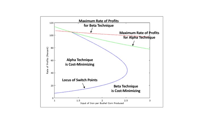
3.3 Bifurcations with Variations in a Coefficient of Production for Iron

Figure 1, at the top of this post, also shows structural changes. The coefficient of production for iron in corn-production varies in the figure. a_1,2 ranges from one to three. The other coefficients of production are as in the reswitching example in Section 3.1 above. And the blue locus shows the rate of profits at switch points.

The example can seen to have structural variations here, also, with three distinct regions for a_1,2, with the same qualitative behavior in each region. For a low enough value of the coefficient of production under consideration, only one switch point exists. The model remains a reswitching example for an intermediate range of this parameter. And for values of this coefficient of production strictly greater than approximately 2.53, the Beta technique is cost-minimizing for all feasible wages and rates of profits.

The maximum rates of profits, for the Alpha and Beta techniques, are also graphed in Figure 1.

4.0 A Story of Technological Process

Using the above example, one can tell a story of technological progress. Suppose at the start of the story, corn production requires a relatively large input of direct labor and iron, per (gross) unit corn produced. Prices of production associated with this technology are such that only one technique is cost-minimizing. For all feasible wages and rates of profits, firms will want to adopt the Beta technique.

Suppose iron production is relatively stagnant, as compared to corn-production. Innovation in the corn industry reduces the labor and iron coefficients defining the single dominant corn-producing process. After some time, either or both coefficients will be reduced enough that the technology for this economy will have become a reswitching example. And around the switch point at the lower wage (and higher rate of profits), a higher wage is associated with the cost-minimizing technique requiring more labor to be hired, in the overall economy, per given bushel of corn produced (net).

But technological innovation continues to proceed apace. At a even lower coefficient of production for the iron input in the corn industry, the structural behavior of the economy changes again. Now a single switch point exists. And the results of the choice of technique around that switch point conforms to outdated neoclassical intuition.

5.0 Conclusion

This example has two properties that I think worth emphasizing.

The choice of technique in the example corresponds to a choice of a production process in the iron industry. As I have told the story, the technology is fixed in iron production. Innovation occurs in corn production. Thus, innovation in one industry can change the dynamics in another industry.

Second, suppose the technology is observed at a single point of time. Suppose the economy is more or less stationary, and that observation is taken at either the start or the end of the above story. Then neither reswitching nor capital reversing will be observed. Yet such phenomena might arise in the future or have arisen in the past.

References

• David Laibman and Edward J. Nell (1977). Reswitching, Wicksell effects, and the neoclassical production function. American Economic Review. 67 (5): pp. 878-888.
• Zonghie Han and Bertram Schefold (2006). An empirical investigation of paradoxes: reswitching and reverse capital deepening in capital theory. Cambridge Journal of Economics. 30 (5): pp. 737-765.
• J. Barkley Rosser, Jr. (1983). "Reswitching as a cusp catastrophe", Journal of Economic Theory. 31: pp. 182-193.
• Bertram Schefold (2013). Approximate surrogate production functions, Cambridge Journal of Economics. 37 (5): pp. 1161-1184.
• Bertram Schefold (2016). Profits equal surplus value on average and the significance of this result for the Marxian theory of accumulation: Being a new contribution to Engels' Prize Essay Competition, based on random matrices and on manuscripts recently published in the MEGA for the first time. Cambridge Journal of Economics. 40 (1): pp. 165-199.

Feels Like Science

Figure 1: Evolution of Two State Variables along Two Dynamic Equilibrium Paths

I continue to explore a micro-founded macroeconomic model from Frank Hahn and Robert Solow, generalized to allow a positive rate of growth of households. Hahn and Solow put forth this model as a strawman, to show that even with perfectly flexible prices and wages, markets clearing always, and rational expectations, room for government macroeconomic management can arise. In their book, they then move on to consider imperfectly competitive markets, norms for wages, and so on.

A dynamic equilibrium path, in the model, defines the values of three state variables at the end of each time period in the model. One of these state variables, the real quantity of money in circulation is easily calculated from the other two. The other two, taken here as the real rate of return on corporate bonds and on money, must be found, in general, by solving a recursive system of two equations at each point in time. I found the code I wrote for this post helpful here.

Figure 1 illustrates the evolution of two state variables for two dynamic equilibrium paths. (The model parameters are β = 2/5, ξ = 2.11, and G = 2. The household utility function is of the form specified by Example 1 in Hahn and Solow, with ε = -1/2.) The stationary, dashed-line, path is for a steady state, which is asymptotically approached by the other dynamic equilibrium path. The oscillations seen in this approach are not in the linear approximation about the steady state. One might view these oscillations as a decaying business cycle. One should be clear, however, that even though economic output varies along such a path, neither unemployment nor disappointed plans arise in this model. Households foresee all future variations in prices and quantities along a dynamic equilibrium path.

One could add various complications to make the model more realistic. Households could live for multiple periods more than two, thereby perhaps modifying the time period for the business cycle. One could add leisure into the utility function and model the supply of labor as the result of trading off the earning of wages for consumption and leisure. Employment would then vary along a business cycle; in this theory, recessions are long vacations. One could add noise terms, from known probability distributions, for various terms. So agents would be continually adjusting their plans to accommodate realizations of stochastic processes. One could add imperfect competition, as modeled by Avinash Dixit and Joseph Stiglitz. I suppose one could describe the parameters of utility functions as lying along a continuum, therefore adding a sort of diversity in the model of households. And so on.

I suppose one would find it difficult to add all of these refinements at once. So one could empirically compare a basic model with each refinement. And a model with one refinement might fit better here and with another there. Room for technical innovation for modelling then arises. Can you add two or more refinements, perhaps simplified, where others could could only add one before? Can you take a model that previously was only described for a linear approximation and analyze at least some non-linearities (as I do above)?

I gather I have just briefly outlined the direction of research in mainstream macroeconomics over the last third of a century, albeit the freshwater school did not start, I take it, with overlapping generations models and a Clower constraint.

None of these refinements would even hint at an approach to addressing the question of how economies get into equilibrium. At the end of each year, the economy is automatically in equilibrium in the model, and this instantaneous magic has been foreseen for all time. Head of households and managers of firms have no need to learn a model of the economy. Agents never have disagreements among themselves about what is the true model. And they never change their minds about the structure of the model. J. R. Hicks, the inventor of the model of temporary equilibrium, came to see that it was set in logical time, not historical time. In other words, John Hicks chose to ally himself with Joan Robinson on this theoretical point.

Without an acceptable understanding of disequilibria, mainstream economists should be tolerant of polyvocality in methodology. Why should some economists not be exploring models that are not microfounded? Why not consider the impact and evolution of social norms, without first insisting that they they be justified by methodological individualism? I consider some work in complexity and agent based modeling to be of interest along these lines and not even all that non-mainstream.

References

Wednesday, October 21, 2015