How To Find Fluke Switch Points

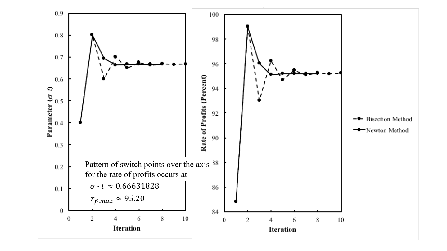
Figure 1: Convergence to a Pattern of Switch Points over the Axis for the Rate of Profits

1.0 Introduction

This post illustrates how to find fluke switch points. As usual, I proceed by example, in this case, as taken from my paper in Structural Change and Economic Dynamics.

2.0 Technoplogy

In this example of a capitalist economy, two commodities, iron and corn, are produced. One process is known for producing iron. In the iron industry, workers use inputs of iron and corn to produce an output of iron. The output of the iron industry is one ton with the inputs shown in Table 1. Two processes are known for producing corn. Each corn-producing process shown in Table 1 produces an output of one bushel corn from inputs of labor power, iron, and corn. Assume constant returns to scale.

Table 1: The Coefficients of Production

Input	Industry
	Iron	Corn
	I	II Alpha	II Beta
Labor	a0,1 = 1	a0,2α = (5191/5770) e1/10 - σt	a0,2β = 305/494
Iron	a1,1 = 9/20	a1,2α = (1/40) e1/10 - σt	a1,2β = 3/1976
Corn	a2,1 = 2	a2,2α = (1/10) e1/10 - σt	a2,2β = 229/494

3.0 Switch Points

I take corn as the numeraire. Wages are paid out of the surplus at the end of the harvest. I take the rate of profits as given. In this post, I do not explain how to find the price of iron and the wage for, say, the Alpha technique, given the technology at a given value of (σ t).

At a switch point, no excess profits or costs arise in evaluating the Beta process in the corn industry at Alpha prices. That is, switch points are the roots of the following equation.

1 - {[p₁^α(σt) a_1,2^β + a_2,2^β](1 + r) + w^α(σt) a_0,2^β} = 0

The above is a quadratic equation for this example. Let f_k(σ t) denote the kth root of the above equation.

r_k = f_k(σ t)

These are the switch points for a specific value of the parameters σ t. I fix σ at 1/10. Figure 2 graphs the switch points, as well as the maxmimum wage, against time. You can see technical progress brings about reswitching and takes it away.

Figure 2: Fluke Switch Points Partition Time

4.0 Numerical Methods

Various fluke cases arise in the example. They can be found by numerical methods. Table 2 defines, for four types of fluke cases, a new function whose root is the parameter values that correspond to the type of fluke case. For illustration, consider the fluke switch point that arises on the axis for the rate of profits with σ t ≈ 0.6663189. That is, g(σ t) is the difference between the maximum rate of profits for the Beta technique and the rate of profits for a selected switch point for the Alpha and Beta techniques.

Table 2: Functions and Their Zeros

Function	Fluke Case
gk(σ t) = fk(σ t) + 1	Pattern of switch points for the reverse substitution of labor.
gk(σ t) = fk(σ t)	Pattern of Switch points over the wage axis.
gk(σ t) = rmax, β - fk(σ t)	Pattern of switch points over the axis for the rate of profits.
gk(σ t) is the discriminant of the quadratic equation above	Reswitching pattern of switch points.

One needs two initial parameter values to start either algorithm specified here. Figure 3 graphs extra profits in operating the corn process in the Beta technique, as evaluated at Alpha prices. Extra profits are shown for two different parameter values. On the left panel, a switch point exists for a rate of profits smaller than the maximum rate of profits. The parameter values are evidently too small for a pattern of switch points over the axis for the rate of profits. On the right panel, the parameter values are too large. These are acceptable initial values.

Figure 3: Initial Values for a Pattern Over the Axis for the Rate of Profits

One can find the desired parameter value by either a bisection method or Newton’s method. Figure 4 provides a flowchart for the bisection method. The parameter values are updated to the midpoint of the current iterations. One of the current iterations is updated while keeping invariant the condition that the current iterations bound the zero of the function whose zero is sought. When the distance between the current iterations is small enough, either iteration is considered an acceptable approximation of the parameter values at which the fluke case arises.

Figure 4: Bisection Method

Figure 5 specifies Newton's method. An iteration for Newton’s method is based on approximating the function whose zero is sought by a straight line going through the two points determined by the previous two iterations. You can see that the slope and intercept for this line are found in the block in the lower left of the figure. And that the next iteration of the parameter values are found by an update calculated with this slope and intercept.

Figure 5: Newton Method

Newton's method is not guaranteed to converge, albeit I have had no issues in this context of finding fluke cases in the analysis of the choice of technique. When it does converge, its convergence is much faster than the bisection method (Figure 1).

Ben Franklin, Proto Marxist

Ben Franklin was one the founding fathers of the United States. He participated in the constitutional convention. He was the first Postmaster General. He did experiments with electricity, when the Leyden jar was a new thing. There is a story about flying a kite in a thunderstorm.

He also wrote about the wealth of nations:

"Finally, there seem to be but three ways for a nation to acquire wealth. The first is by war, as the Romans did, in plundering their conquered neighbors. This is robbery. The second by commerce, which is generally cheating. The third by agriculture, the only honest way, wherein man receives a real increase of the seed thrown into the ground, in a kind of continual miracle, wrought by the hand of God in his favour, as a reward for his innocent life and his virtuous industry."

I find an echo of Francois Quesnay and the physiocrats in the above quotation. He was also a proponent of a labor theory of value:

"Trade in general being nothing else but the exchange of labor for labor, the value of all things is justly measured by labor."

I could not find Franklin in the index of Marx's Theories of Surplus Value. A quick google search had me stumbling upon Aiken's 1966 article.

References

• John R. Aiken. 1966. Benjamin Franklin, Karl Marx, and the Labor Theory of Value. The Pennsylvania Magazine of History and Biography 90 (3): 378-384.

An Intensive Rent Example From Freni

Figure 1: A Pattern Diagram

1.0 Introduction

Aside, perhaps from the above visualization, nothing novel is presented in this post. It follows an example presented by Freni (1991). I know of this example from problems 7.7 and 7.29 in Kurz and Salvadori (1995). The oddities of this example can be seen in an earlier and more complicated example from D'Agata (1983).

This is an example of intensive rent. When the requirements for use are large enough, capitalists will use more than one process to produce a commodity on homogeneous land. The scarcity of land is expressed in the emergence of rent. This example, though, is a challenge to Sraffa's work. The cost-minimizing technique is a unique function of the wage, but it is not a unique function of the rate of profits. The wage frontier is not downward sloping. How disappointing.

2.0 Technology and Requirements for Use

This is an example (Table 1) of a capitalist economy in which one commodity, corn, is produced by laborers working with inputs of (seed) corn on one type of homogeneous land. Twenty four acres (T = 24) of land are assumed available, and three processes are known for producing corn Each process exhibits constant returns to scale (CRS), up to the limit imposed by the given quantity of land.

Table 1: The Coefficients of Production

Input	Process
	I	II	III
Labor	a0,1 = 2/5	a0,2 = 2	a0,3 = 1
Land	c1,1 = 1/5	c1,2 = 1/2	c1,3 = 1/7
Corn	a1,1 = 7/10	a1,2 = 7/24	a1,3 = 21/32

In this example, requirement for use, also known as net output, is d = 35 bushels. I also take the net output as the numeraire.

3.0 Quantity Flows

I analyze six possible techniques of production. In each of the Alpha, Beta, and Gamma techniques, only one process is used to produce corn. Table 2 shows the gross output of each process needed to satisfy the requirements for use. Notice the Beta technique requires more land than is available; it is infeasible.

Table 2: Techniques of Production

Technique	Process			Acres Used
	I	II	III
Alpha	qα,1 = 350/3	0	0	70/3 ≈ 23.3
Beta	0	qβ,2 = 840/17	0	420/17 ≈ 24.7
Gamma	0	0	qγ,3 = 1120/11	160/11 ≈ 14.5
Delta	qδ,1 = 60	qδ,2 = 24	0	24
Epsilon	qε,1 = 3640/29	0	qε,3 = -224/29	24
Zeta	0	qζ,2 = 4368/95	qζ,3 = 672/95	24

In each of the Delta, Epsilon, and Zeta techniques, two processes are applied, side-by-side, in farming the land. Table 2 shows the gross outputs for these techniques, too. Notice that if the Epsilon technique were adopted, the third process would need to run at a negative level. The Epsilon process is infeasible.

So for the given technology, acres of land, and requirements for use, the Alpha, Gamma, Delta, and Zeta techniques are feasible. Which techniques are feasible varies with the requirements for use.

3.1 Alpha Technique

I might as well give some indication of how quantity flows are found. Accordingly, suppose the Alpha technique is adopted. The gross output of the first process is found by solving the following equation:

d = q_α,1 - a_1,1 q_α,1 = (1 - a_1,1) q_α,1

The amount of land farmed is c_1,1 q_α,1. The technique is feasible only if this amount does not exceed the given amount of land available.

3.2 Delta Technique

On the other hand, suppose the Delta technique is applied. The first process is operated alongside the second process. The gross outputs of the two processes must be such that the land is totally farmed:

c_1,1 q_δ,1 + c_1,2 q_δ,2 = T

The gross outputs must also be such that the requirements for use are satisfied.

d = (q_δ,1 + q_δ,2) - (a_1,1 q_δ,1 + a_1,2 q_δ,2)

The above is a system of two linear equations in two unknowns, q_δ,1 and q_δ,2. Nothing guarantees that in the solution, the levels of gross output must be positive. If they are negative, the technique is infeasible.

4.0 Price Equations

The cost-minimizing technique, at a given rate of profits, depends on prices.

4.1 Alpha Technique

Suppose the Alpha technique is adopted. The land is not fully farmed. Since it is in excess supply, it pays no rent. The parameters for the first process yield an equation.

p_α a_1,1 (1 + r) + w_α a_0,1 = p_α

I stated above that net output is the numeraire.

p_α d = 1

One can solve the above system to obtain the wage as a function of the rate of profits. The wage curve for the Alpha technique is downward-sloping.

4.2 Delta Technique

Because of the scarcity of land, a positive rent emerges for the delta technique. The parameters for the two operated processes provide two equations for the system of prices of production:

p_δ a_1,1 (1 + r) + ρ_δ c_1,1 + w_δ a_0,1 = p_δ

p_δ a_1,2 (1 + r) + ρ_δ c_1,2 + w_δ a_0,2 = p_δ

As usual, the specification of the numeraire yields another price equation.

p_α d = 1

I want to make a start towards solving the above system. One can multiply the first equation by (1/c_1,1), the second equation by (1/c_1,2), and subtract the second from the first:

[a_1,1/(dc_1,1) - a_1,2/(dc_1,2)] (1 + r) + w_δ[a_0,1/c_1,1 - a_0,2/c_1,2] = [1/(dc_1,1) - 1/(dc_1,2)]

Notice that the rent of land has been eliminated. Land, in Sraffian terminology, is a non-basic commodity. The system of equations can be solved seperately for the wage and prices as a function of the rate of profits. Then rent can be found afterwards.

This structure also suggests taxing rent of land has no further consequences on the price system. At least some followers of Henry George should investigate the role of land and non-basic commodities in post-Sraffian price theory.

5.0 Choice of Technique

Figure 2 graphs the wage curves and rent, for feasible techniques for this example, with the specified requirements for use, against the rate of profits. For techniques in which two processes are activated on the homogeneous land, the wage curves in the panel on the left are only shown where rent is non-negative.

Figure 2: Wage Curves and the Frontier

I indicate the cost-minimizing technique(s) with heavy lines in the above figure. Notice that for a range of profits of approximately 13.3 percent and 24.7 percent, the Alpha, Delta, and Zeta techniques are all cost-minimizing. The choice of technique is not unique. Furthermore, for a rate of profits above this range, no technique is cost-minimizing. This result would have been surprising to Sraffa, as I read him.

The wage frontier, in this case, is not the outer frontier of wage curves. Nor is it the inner frontier. So I want to say something about how the choice of technique is analyzed here.

The wage and the price of corn, as determined by the Alpha technique, can be used to evaluate the costs and revenues, of operating each of the three processes in the technology, at a unit level. The costs include the given rate of profits. The left panel in Figure 3 shows the difference between such revenues and costs. That is, it shows what are known as extra profits in activating each process. Notice that no extra profits are to be made in operating the first process, thus confirming that the price system has been solved correctly. For rates of profits below the first switch point shown, no extra profits can be made by activating the second or third process; Alpha is cost minimizing in this range. For a higher rate of profits, extra profits can be made by activating the second process. Alpha is no longer cost-minimizing.

Figure 3: Extra Profits for the Alpha and Gamma Techniques

The right panel repeats the analysis for the price system for the Gamma technique. For the full range of feasible rates of profits, no extra profits are obtained by operating the third process, as expected. But extra profits can always be made, at Gamma prices, by operating the first or second process; Gamma is never cost-minimizing.

Figure 4 repeats the analysis for the Delta and Epsilon techniques. The costs now include rents. Only one of three processes available makes extra profits or incurs costs greater than revenues. The range of the rate of profits in which each of these techniques is cost-minimizing is indicated.

Figure 4: Extra Profits for the Delta and Epsilon Techniques

6.0 Ricardian Dynamics

The above has shown how to find wage(s), prices, and rent, for a given requirements for use. Consider the full range of feasible net outputs. Ricardo told a story, using prices of production (not his terminology) of how the types of land and activated processes vary with an increase in requirements for use. This story involves wages, population, and his advocacy against the corn laws. Anyway, Figure 1, at the top of this post, illustrates aspects of Ricardian dynamics in this numeric example.

For a small enough level of net output, land need not be wholly farmed and is in excess supply. The choice of technique can be found by constructing the outer frontier out of the wage curves for the Alpha, Beta, and Gamma technique. For a small rate of profits, the Alpha technique is cost-minimizing, while for a larger rate of profits, the Beta technique is cost-minimizing. All wage curves and the outer frontier are downward-sloping, as in part I of Sraffa (1960).

For a large enough level of net output, but at a still feasible level, the Gamma, Epsilon, and Zeta techniques are the only feasible techniques. Under Epsilon and Zeta, the first and second processes, respectively, are combined with the third process so as to ensure that only the amount of land available is farmed. The choice of technique is found from the inner frontier of the wage curves. For a small rate of profits, the Epsilon technique is cost-minimizing, and the Zeta technique is cost-minimizing at a high rate of profits. All wage-curves are downward sloping. This example of intensive rent resembles a well-behaved model of extensive rent.

The difficulties and surprises arise for an intermediate level of net output, as described above.

7.0 Conclusion

I do not fully know what to make of this example. I notice that the cost-minimizing technique is uniquely determined (except at switch points) by the wage. And it is analyzed by techniques developed by Sraffa and his followers. I can further apply by approach of perturbing parameters, if I want. Nevertheless, it reveals some of the disappointments arising from the theory of joint production.

References

• D'Agata, A. 1983. The existence and unicity of cost-minimizing systems in intensive rent theory. Metroeconomica 35: 147-158.
• Freni, G. 1991. Capitale technico nei modelli dinamici ricardiani. Studi Economici, 44: 141-159.
• Kurz and Neri Salvadori. 1995. Theory of Production: A Long-Period Analysis, Cambridge University Press.

Elsewhere

John Eatwell On The Bomb Sraffa Planted At The Foundations Of Economics

• James Galbraith on Dismal Economics, reviewing books by Mason Gaffney and Fred Harrison, Stephen Marglin, Alessandro Roncaglia, and Robert Skidelsky.
• Jane Gleeson-White, in the Guardian, on accounting, unpaid care work, and the biosphere.
• A blog post pointing out Bob Murphy's confusions and mistakes on the implications of the Cambridge Capital Controversy for the Austrian school. Compare and contrast with here.

What Is Socially Necessary Abstract Labor Time?

To me, this is an easy question. SNALT, for a capitalist economy, is:

L = a₀ (I - A)^-1 y

The notation is from Luigi Pasinetti's Lectures on the Theory of Production. The idea can be empirically applied with data from national income and product accounts (NIPAs), using techniques explained in, for example, Ronald Miller and Peter Blair's Input-Output Analysis

Extensive Rent For A Reswitching Example

Figure 1: Wage Curves and Rent

1.0 Introduction

I might as well illustrate an example with extensive rent and reswitching. I find it incredible that the agents in these sorts of models understand the implications of, say, a variation of the distribution of income for their self-interests. Nevertheless, I try to note the consequences of variation in the distribution of income and perturbations of model parameters on prices of production. And I do not worry too much about disequilibria.

2.0 Technology and Requirements for Use

Consider a capitalist economy in which two commodities, iron and corn, are produced. One process is known for producing iron. In the iron industry, workers use inputs of iron and corn to produce an output of iron. The output of the iron industry is one ton with the inputs shown in Table 1. Two processes are known for producing corn. Each corn-producing process operates on a specific type of land. The coefficients of production shown in Table 1 are for an output of one bushel corn. These processes can be thought of as examples of joint production. Their outputs are corn and the same quantity of land used as input, unchanged by the production process. Presumably, some of the labor in these processes is used to maintain the land in a given state. For this post, I assume σt is 17/100.

Table 1: The Coefficients of Production

Input	Iron Industry	Corn Industry
	I	II	III
Labor	a0,1 = 1	a0,2 = 5191/5770	a0,3 = (305/494) e(3/20) - σt
Type 1 Land	0	c1,2 = 1	0
Type 2 Land	0	0	c2,3 = e(3/20) - σt
Iron	a1,1 = 9/20	a1,2 = 1/40	a1,3 = (3/1976) e(3/20) - σt
Corn	a2,1 = 2	a2,2 = 1/10	a2,3 = (229/494) e(3/20) - σt

The specification of technology is completed by noting the values of parameters for the quantities available of non-produced means of production. For this numerical example, let there be 100 acres of type 1 land and 100 acres of type 2 land. The iron-producing process and each corn-producing process exhibits constant returns to scale, up to the limits imposed by the endowments of land.

I consider stationary states with a net output consisting solely of corn. A bushel corn is the numeraire. Any one of four techniques can be used to produce corn, depending on the requirements for use. The process for producing iron is part of each technique. Table 2 specifies which types of land are fully or partially farmed in each technique. In the Alpha and Beta techniques, both types of land are cultivated, with one type only partially farmed. In the remaining two techniques, one type of land is left totally farrow. Which techniques are feasible depends on the endowments of the land and on the requirements for use.

Table 2: Techniques

Technique	Type of Land
	Type 1	Type 2
Alpha	Fully farmed	Partially farmed
Beta	Partially farmed	Fully farmed
Gamma	Partially farmed	Farrow
Delta	Farrow	Partially farmed

Suppose requirements for use, that is, net output of corn, exceed 55.112 bushels and fall below 80.90. Delta is not feasible. Beta and Gamma are feasible. With Alpha, corn is in excess supply.

2.0 Prices of Production

I have asserted above that only the Beta and Gamma techniques are feasible, given technology, endowments, and requirements for use. A system of prices of production is associated with each technique. For Beta, type 2 land pays a rent. For Gamma, neither type of land pays a rent.

3.1 Prices for Beta

Suppose managers of firms have adopted the Beta technique. Prices of production satisfy the following system of three equations:

(p_β a_1,1 + a_2,1)(1 + r) + w_β a_0,1 = p_β

(p_β a_1,2 + a_2,2)(1 + r) + w_β a_0,2 = 1

(p_β a_1,3 + a_2,3)(1 + r) + ρ₂ c_{2, 3} + w_β a_0,3 = 1

In these equations, p_β is the price of iron, w_β is the wage, ρ₂ is the rent per acre for type 2 land, and r is the given rate of profits. The left-hand side (LHS) of each equation is the cost of operating the corresponding process at a unit level. Costs include the cost of previously produced commodities used as raw material or ancillary inputs, the going rate of profits on these costs, rent, and wages. Since type 1 land is not fully cultivated, it obtains no rent. The right-hand side (RHS) is the revenue obtained from the corresponding process.

For prices of production, costs do not exceed revenue for any operated process. Furthermore, supernormal profits cannot be made in any prices.

3.2 Prices for Gamma

Now suppose instead that the Gamma technique is adopted by managers. Prices of production, in analogous notation, must satisfy the following system of equalities and inequalities:

(p_γ a_1,1 + a_2,1)(1 + r) + w_γ a_0,1 = p_γ

(p_γ a_1,2 + a_2,2)(1 + r) + w_γ a_0,2 = 1

(p_γ a_1,3 + a_2,3)(1 + r) + w_γ a_0,3 > 1

3.3 The Choice of Technique

Which system of equations and inequalities prevails for a given rate of profits. The analysis of the choice of technique, in models of extensive rent, can still be based on wage curves. In both the Beta and the Gamma techniques, the first two equations for prices of production are in three variables: the price of iron, the wage, and the rate of profits. Thus, one can solve for the wage as a function of the rate of profits. This is the curve labeled 'Type 1 Land' in the left panel in Figure 1 above.

For the Beta technique, one can solve the last equation for the rent on type 2 land, given the solution from the first two equations. This decomposition of the equations shows that land is a non-basic commodity, in Sraffa's terminology. Hence, a tax on land will not affect the price of iron.

The wage curve for type 2 land can be found from the system of equalities and inequalities for the Delta technique. This wage curve is also shown in Figure 1.

Consider the outer frontier of the wage curves in Figure 1. If requirements for use can satisfied by only cultivating that type of land, then the cost-minimizing technique at a given rate of profits is the corresponding technique. That is, Gamma is cost-minimizing for rates of profits between the switch points.

If the technique for the wage curve on the frontier is not feasible, the corresponding type of land will be fully cultivated. To find the cost-minimizing technique drop down to next wage curve at the given rate of profits. In this example, the cost-minimizing technique corresponds to the wage curve on the inner frontier of the wage curves. So Beta is cost-minimizing at low and high rates of profits. The same rate of profits is made in operating both type 1 and type 2 land, and type 2 land pays a rent.

Whether or not type 2 land is introduced into cultivation alongside partial cultivation of type 1 land depends on the rate of profits. When type 2 land is fully cultivated, less of type 1 land is farmed.

4.0 Conclusion

Type 1 land is partially farmed. Whether or not type 2 land is fully farmed or left farrow depends on distribution. For high and low rates of profits (or low and high wages), type 2 land is fully farmed and owners of type 1 land receive a rent. For intermediate rates of profits (or wages), type 2 land is left farrow, and no land receives a rent.

Employment is greater under Gamma than when the Beta technique is adopted. Thus, around the switch point at the lower wage, an increased wage is associated with each worker benefitting and employment being increased. Owners of type 2 land have a stake in how the social question is being decided among workers and capitalists.

Some Difficulties In Reading Marx

"Let us take the process of circulation in a form under which it presents itself as a simple and direct exchange of commodities. This is always the case when two owners of commodities buy from each other, and on the settling day the amounts mutually owing are equal and cancel each other. The money in this case is money of account and serves to express the value of the commodities by their prices, but is not, itself, in the shape of hard cash, confronted with them. So far as regards use-values, it is clear that both parties may gain some advantage. Both part with goods that, as use-values, are of no service to them, and receive others that they can make use of. And there may also be a further gain. A, who sells wine and buys corn, possibly produces more wine, with given labour-time, than farmer B could, and B on the other hand, more corn than wine-grower A could. A, therefore, may get, for the same exchange-value, more corn, and B more wine, than each would respectively get without any exchange by producing his own corn and wine. With reference, therefore, to use-value, there is good ground for saying that 'exchange is a transaction by which both sides gain.'" -- Karl Marx, Capital, Chapter 5: Contradictions in the General Formula of Capital.

The sheer volume of his work makes Karl Marx difficult to read. Here I concentrate on the three volumes of Capital. In the Progress Publishers edition, they consist of 867 pages, 551 pages, and 948 pages, respectively. Is there a one-semester class in which students are expected to read all of that? If I were a scholar, I suppose I would be required to learn German. I suppose one ought to also look at the secondary and tertiary literature, maybe from one's home country. (The fact that I can assume such literature exists, wherever you are coming from, attests to Marx's importance.)

Another difficulty is in understanding why Marx chose his order of exposition. The introduction to the Grundrisse is an important text on method here, although I gather Marx came to think of the order in the main text of the Grundrisse as backwards. As I understand it, Marx works from higher levels of abstraction to lower levels, with the concrete being overdetermined, in some sense. These levels are supposed to be real abstractions. Reality is not generated out of thought, as in Hegel. One might respond to the first objection here by saying that the distinction between fixed and circulating capital is a volume 2 issue and can be ignored in volume 1. The overall arc is to consider production in volume 1, circulation combined rather mechanically with production in volume 2, and then the unity of production and circulation in volume 3. The decomposition of surplus value into profits, interest on monetary loans, rent, wages for non-productive workers (such as clerks hired by banks or lawyers) cannot be fully explained until volume 3. And Marx never even gets to taxes and the state. But, according to Lenin, I do not understand Capital since I have never read Hegel's Logic, as one might expect of one who has read some of Bertrand Russell.

Capital is an immanent critique, and it is not always easy to be sure of Marx's attitude to what he is writing about. I think that Marx does not expect prices of production to be proportional to labor values, for example. He says as much in a footnote at the end of chapter 5 in volume 1. It does not help the reader that he does not explain this as fully as he ever will until towards the start of volume 3, more than a thousand pages later. The distinction between labor values and exchange values seems to be of no matter in much of the middle of volume 2, where he explains how the wear and tear of long-lived machinery, the value of ancillaries such as fuel to keep machinery running and to light a factory, and raw materials that actually appear changed in the product all contribute to a commodity's value.

I think a major difficulty some have is that a Marx is developing a systems view or structural approach, in some sense. I find many bourgeois commentators seem to object to the labor theory of value based on the feelings of those engaged in a single transaction or on a supposed analysis of a single market. This standpoint seems besides the point to me. When, in volume 1, Marx talks about the capitalist, he is treating the capitalist as "capital personified", and so on.

I think a major point of Marx is why so many have necessary illusions about capitalism. So many perceive human social powers as relationships inherent in objects, such as money capital goods, or land, or inherent in institutions such as markets. This confusion and fetishism by apologists, at a superstructural level, has a role in keeping capitalism going. Marx tries to explain such illusions created by markets.

An issue I have is with readings of Marx as presenting a scientific, positivistic theory of prices and distribution. Even if not fully in the spirit of Marx, I find empirical work with input-output tables of interest, though.

Structural Dynamics With Extensive Rent

Figure 1: Variation in Switch Points with Time

1.0 Introduction

This post continues my effort to understand how fluke cases can partition parameter spaces in models of prices of production with extensive rent. Some background for this post is here, here, and here.

2.0 Technology

The technology is described by the coefficients of production in Table 1. I assume that requirements for use are such that they cannot be satisfied by cultivating only two types of land. After fully cultivating two types, the third type must also be introduced into cultivation, at least partially. See this post for a slightly longer description of the technology.

Table 1: The Coefficients of Production

Input	Iron Industry	Corn Industry
	I	II	III	IV
Labor	a0,1 = 1	a0,2 = 1/2	a0,3 = 3	a0,4(t) = 2.0743 e-0.03648 t
Type 1 Land	0	b1,2 = 1	0	0
Type 2 Land	0	0	b2,3 = 1	0
Type 3 Land	0	0	0	b3,4 = 1
Iron	a1,1 = 0	a1,2 = 1/2	a1,3 = 1/8	a1,4(t) = 0.3551 e-0.06337 t
Corn	a2,1 = 1/2	a2,2 = 0	a2,3 = 0	a2,4(t) = 0.3343 e-0.2906 t

Table 2 lists the techniques for this example. Feasiblity of a technique is determined by requirements for use. Only techniques in which all three types of land must be cultivated are listed.

Table 2: Techniques

Technique	Type of Land
	Type 1	Type 2	Type 3
Alpha	Fully farmed	Fully farmed	Partially farmed
Beta	Partially farmed	Fully farmed	Fully farmed

3.0 Prices

I consider the system of prices of production. Profits, rent and wages are paid out of the surplus at the end of the year. Each of the four processes contributes an equation to the system of price equations. A bushel corn is the numeraire, and rent must be zero on at least one type of land.

4.0 Variations of the Choice of Technique

In Figures 1 and 2, thin vertical lines partition time into numbered regions. In each numbered region, the variation of the cost-minimizing technique with distribution is qualitatively invariant. The partitions are labeled with a type of patterns of switch points. Region 8 is a narrow range of time between a pattern for the r-order of fertility, which occurs first, and a pattern over the axis for the rate of profits for the order of rentability.

Figure 2: Variation in Switch Points with Time (Start Enlarged)

The maximum rate of profit, the rate of profits at switch points, and the rate of profits for which the rent per acre for the two types of land that pay rent are equal are plotted as functions of time. Heavy solid lines, aside from the bound on the infeasible region, are for switch points on the inner frontier of the wage curves. These solid lines bound areas in which the cost-minimizing technique, Alpha, Beta, or Gamma, is as shown. Dashed lines are for switch points on the outer frontier. For each technique, the dashed lines bound areas in which the order of fertility does not change. Dotted lines are for the rate of profits at which rents are equal. The dashed lines bound areas, for each technique, in which the order of rentability is invariant. Table 3 summarizes how, within each numbered region, the choice of technique, the order of fertility, and the order of rentability vary with the rate of profits.

Table 3: Description of Partitions with Rate of Profits Given

Region	Range of r	Technique	Order of Fertility	Order of Rentability
1	0 < r < r1,2	Alpha	1 ,2, 3	ρ1 > ρ2 > 0. ρ3 = 0
	r1,2 < r < rmax, 3			ρ2 > ρ1 > 0. ρ3 = 0
2	0 < r < r1,2	Alpha	1 ,2, 3	ρ1 > ρ2 > 0. ρ3 = 0
	r1,2 < r < r*			ρ2 > ρ1 > 0. ρ3 = 0
	r* < r < rmax, 3		2, 1, 3
3	0 < r < r1,2	Alpha	1 ,2, 3	ρ1 > ρ2 > 0. ρ3 = 0
	r1,2 < r < r*			ρ2 > ρ1 > 0. ρ3 = 0
	r* < r < r**		2, 1, 3
	r** < r < rmax, 1	Beta	2, 3, 1	ρ2 > ρ3 > 0. ρ1 = 0
4	0 < r < r*	Gamma	1 ,3, 2	ρ1 > ρ3 > 0. ρ2 = 0
	r* < r < r1,2	Alpha	1 ,2, 3	ρ1 > ρ2 > 0. ρ3 = 0
	r1,2 < r < r**			ρ2 > ρ1 > 0. ρ3 = 0
	r** < r < r***		2, 1, 3
	r*** < r < rmax, 1	Beta	2, 3, 1	ρ2 > ρ3 > 0. ρ1 = 0
5	0 < r < r1,3	Gamma	1 ,3, 2	ρ1 > ρ3 > 0. ρ2 = 0
	r1,3 < r < r*			ρ3 > ρ1 > 0. ρ2 = 0
	r* < r < r**		3, 1, 2
	r** < r < r2,3	Beta	3 ,2, 1	ρ3 > ρ2 > 0. ρ1 = 0
	r2,3 < r < r***			ρ2 > ρ3 > 0. ρ1 = 0
	r*** < r < rmax, 1		2, 3, 1
6	0 < r < r1,3	Gamma	1 ,3, 2	ρ1 > ρ3 > 0. ρ2 = 0
	r1,3 < r < r*			ρ3 > ρ1 > 0. ρ2 = 0
	r* < r < r**		3, 1, 2
	r** < r < r2,3	Beta	3 ,2, 1	ρ3 > ρ2 > 0. ρ1 = 0
	r2,3 < r < rmax,1			ρ2 > ρ3 > 0. ρ1 = 0
7	0 < r < r*	Gamma	1 ,3, 2	ρ3 > ρ1 > 0. ρ2 = 0
	r* < r < r**		3, 1, 2
	r** < r < r2,3	Beta	3 ,2, 1	ρ3 > ρ2 > 0. ρ1 = 0
	r2,3 < r < rmax,1			ρ2 > ρ3 > 0. ρ1 = 0
8	0 < r < r*	Gamma	3, 1, 2	ρ3 > ρ1 > 0. ρ2 = 0
	r* < r < r2,3	Beta	3 ,2, 1	ρ3 > ρ2 > 0. ρ1 = 0
	r2,3 < r < rmax,1			ρ2 > ρ3 > 0. ρ1 = 0
9	0 < r < r*	Gamma	3, 1, 2	ρ3 > ρ1 > 0. ρ2 = 0
	r* < r < rmax,1	Beta	3 ,2, 1	ρ3 > ρ2 > 0. ρ1 = 0

Some of the fluke cases that partition the parameter space in this example arise in models with circulating capital alone and no scarce unproduced means of production. Some are specific to models with land. At the time for the partition between regions 2 and 3, a fluke switch point between the Alpha and Beta techniques occurs on the inner wage frontier with a wage of zero. This fluke is associated with the emergence of a range of low rates of profits in which the Beta technique is cost-minimizing. The partition between regions 3 and 4 is characterized by a fluke switch point on the inner wage frontier with a rate of profits of zero. This fluke is associated with the emergence of a range of high rate of profits in which the Gamma technique is cost-minimizing.

The three-technique pattern of switch points, defining the partition between regions 4 and 5, is probably the most visually noticeable fluke case depicted in Figure 8. For the coefficients of production at this instant in time, the wage curves for the Alpha, Beta, and Gamma techniques intersect at a single switch point. This switch point is simultaneously on the inner and the outer frontiers of the wage curves. For the rate of profits at which this switch point is defined, all three types of lands are equally fertile, and none of them pay any rent. None of the types of land need be fully cultivated prior to some other type being taken into cultivation.

Fluke cases I christen patterns for the r-order of fertility are specific to models of rent. A fluke switch point on the outer frontier also lies on the wage axis at the time which partitions regions 7 and 8. At this time, the range of the rate of profits in which the order of fertility is type 1, type 3, and type 2 land vanishes over the wage axis. The partition between regions 1 and 2 qualitatively resembles the partition between regions 5 and 6. A switch point on the outer frontier of wage curves occurs at a rate of profits of 100 percent, which is also the maximum rate of profits of the Beta technique. This fluke case is associated with a disappearance of a range of the rate of profits at which the order of fertility is type 2, type3, and type 1 lands.

A pattern for the w-order of fertility occurs at a time of approximately 6.0619. The switch point between type 1 and type 3 lands of the outer occurs at the same wage as the maximum wage for type 2 land. This switch point is associated with the disappearance of a range of wages at which the order of fertility is type 3, type 1, and type 2 lands, given the wage. Since the rate of profits is taken as given throughout this post, this example of a pattern for the w-order of fertility is merely an aside.

Patterns in the order of rentability are also specific to models with land. Consider the partition between regions 6 and 7. This is a pattern over the wage axis for the order of rentability. At a rate of profits of zero, the rent on an acre of type 1 and type 3 land is identical. This fluke case is associated with the disappearance of a range of the rate of profits in which the order of rentability is type 1, type 3, type 2 lands. The partition between regions 8 and 9 is a pattern over the axis for the rate of profits for the order of rentability.

5.0 Conclusions

This post continues to extend my research program. It illustrates that a divergence between the order of fertility and the order of rentability is not a fluke case.

Background Needed For Debates On The Labor Theory Of Value Versus Marginalism

A Propertarian Getting The Better Of The Wrong Side Of The Argument

I have been looking at some debates on YouTube. Not only is there a culture of twitch streamers debating. There are some, such as Noah Cortez "Booksmarts", critiquing debates. By the way, here is a video providing an overview of (Resnick and) Wolff's academic work, seemingly inspired by the prominence Wolff is gaining with his YouTube presence.

I suppose that this post is aspirational, and some of these points can be argued over. I guess, this post is related. I'd like for the debaters to:

• Recognize that such a debate topic is orthogonal to a debate on socialism versus capitalism. Thus, Barone's economic calculation problem is not on-topic, without an argument.
• Know the distinction between use value and exchange value, as in Aristotle (arguably), Adam Smith, Ricardo, and Marx. Use value is about physical properties of commodities, not preferences or utility functions.
• Know something of the theory of revealed preference, ordinal utility, and cardinal utility.
• Distinguish between market prices and natural prices, also known as prices of production. Prices of production are defined when outputs are at the level of what Adam Smith calls effectual demand.
• Distinguish between the short run and long run in, for example, Marshall. Some, maybe, should know that Mises' evenly rotating economy is compatible with an analysis of prices of production. Walras' general equilibrium is a theory of the long run.
• Recognize prices of production are consistent with utility maximization, as in marginalism.
• Distinguish prices of production from embodied labor values, also known as employment multipliers. Maybe debaters should be able to contrast labor values with labor commanded.
• Recognize supply and demand are not functions of price in Smith, Ricardo, and Marx, but are such in marginalism. Well-defined functions for supply and demand were abandoned, more or less, in marginalist long run theory after the CCC.
• Understand that variations of organic composition of capital suggests, as explained by Marx in his account of the transformation problem, that prices of production cannot be expected to be proportional to labor values.
• Known that Marx claimed, in Volume 3, that the rate of profits used in calculating prices of production comes from the system of labor values. Max also claimed that total prices and total profits were equal to total labor values and total surplus values, or so I think. I call these some of Marx's invariants.
• Have some familiarity with national income accounting and Leontief matrices.
• Have some awareness of empirical results on the labor theory of value as a theory of price.
• Have some awareness of empirical results on trends in the OCC, the rate of exploitation, and the rate of profits.
• Have some view on what empirical results test marginalism. Does behavioral economics show that it is both falsifiable and false?

By the way, I do not have a high opinion of Böhm-Bawerk's Karl Marx and the Close of his System.

On My Research Program

"I know not how I may seem to the world, but as to myself I seem to have been only like a boy playing on the sea-shore and diverting myself in now and then finding a smoother pebble or a prettier shell than ordinary, whilst the great ocean of truth lay all undiscovered before me." -- Isaac Newton (apocryphal?)

For the past couple of years, I have been pursuing a research program that I seem to have stumbled upon. I am looking for fluke switch points, where these fluke switch points partition certain parameter spaces. The analysis of the choice of technique is supposed to be qualitatively invariant, in some sense, in each region formed by these partitions, but varies among regions.

I have tried to define a taxonomy for such fluke switch points. Using an example, I have explored structural dynamics. Analyzing fluke switch points in models of fixed capital lets me see maybe more deeply into the incoherence of Austrian and marginalist approaches. Lately, I have been considering a parameter space of relative markups. Even more recently, I have been considering models of extensive rent.

Mathematically, these post-Sraffian models I have been exploring are open. Given parameters characterizing the technology and relative markups among industries, the distribution of income can vary with one degree of freedom. But if the wage, for example, and the size and composition of the net product is given, the rate of profits and the price of each commodity is determined. This is a matter of mathematics, close to accounting. Is my approach compatible with Ajit Sinha's reading of Sraffa's work as an approach akin to geometrical reasoning?

I do not know that Tony Lawson would accept that these models are ontologically open in his sense. Similarly, Nicholas Georgescu-Roegen made a distinction between what he called arithmorphic and dialetic reasoning. In my approach, I emphasize how quantitative perturbations of parameters leads to qualitative change in admittedly static models. I limit myself to discovering structures at the level of mesoeconomics, not visible at the level of individual transactions or an individual (non-vertically integrated) industry.

I rarely comment on whether or not I am taking an empirical economy as given. My approach certainly relates to Leontief input-output matrices, which can be constructed or approximated from National Income and Product Accounts (NIPAs). The econometrician would probably also want prices indices for individual industries. At a given point of time, one might say a process is dominant in each industry. But some firms might be still operating old processes, and others might be introducing new processes with which they hope to make super normal profits for a time. This observation provides some justification for considering the choice of technique. I often postulate continuous declines in coefficients of production, following Pasinetti's lead, or variations in relative markups. Is this a matter of counter-factual reasoning that Sraffa would reject?

I am aware that my models are not set in historical time. This is a point of contention for some Post Keynesian, such as Lars Syll. Do at least some of my partitions have implications for the dynamics of how or whether market prices approach prices of production? This is a question that I will continue not to address. I found intriguing this talk by Ian Wright, with accompanying handout.

Research in flukes may lead to more acceptance of possibility of reswitching, capital reversing, reverse substitution of labor, recurrence of processes. I wonder if somebody that understands something about algebraic geometry could summarize my approach more shortly, but even more abstractly. I hope and wish that I can read sometime somebody extending this research. Some sort of structures definitely seem to exist in these parameter spaces.

Fluke Cases for the Order of Fertility

Figure 1: Wage Curves for Fluke Case for r-Order of Fertility

1.0 Introduction

This post illustrates two fluke cases that can arise in a model with land and extensive rent. I call these a pattern of switch points for the r-order of fertility and a pattern of switch points for the w- order of fertility. I have previously described a fluke case in the order of rentability, which can be either over the wage axis or over the axis for the rate of profits. These fluke cases can arise in an analysis in which a parameter space is partitioned by fluke cases such that in each of the resulting regions the analysis of the choice of technique does not qualitatively vary, in some sense.

2.0 Technology

The technology is described by the coefficients of production in Table 1. Let there be T₁ = 100 acres of type 1 land, T₂ = 80 acres of type 2 land, and T₃ = 40 acres of type 3 land. See this post for a slightly longer description of the technology.

Table 1: The Coefficients of Production

Input	Iron Industry	Corn Industry
	I	II	III	IV
Labor	a0,1 = 1	a0,2 = 1/2	a0,3 = 3	a0,4(t) = 2.0743 e-0.03648 t
Type 1 Land	0	b1,2 = 1	0	0
Type 2 Land	0	0	b2,3 = 1	0
Type 3 Land	0	0	0	b3,4 = 1
Iron	a1,1 = 0	a1,2 = 1/2	a1,3 = 1/8	a1,4(t) = 0.3551 e-0.06337 t
Corn	a2,1 = 1/2	a2,2 = 0	a2,3 = 0	a2,4(t) = 0.3343 e-0.2906 t

Table 2 lists the techniques for this example. Feasiblity of a technique is determined by requirements for use.

Table 2: Techniques

Technique	Type of Land
	Type 1	Type 2	Type 3
Alpha	Fully farmed	Fully farmed	Partially farmed
Beta	Partially farmed	Fully farmed	Fully farmed
Gamma	Fully farmed	Partially farmed	Fully farmed
Delta	Fully farmed	Partially farmed	Fallow
Epsilon	Fully farmed	Fallow	Partially farmed
Zeta	Partially farmed	Fully farmed	Fallow
Eta	Fallow	Fully farmed	Partially farmed
Theta	Partially farmed	Fallow	Fully farmed
Iota	Fallow	Partially farmed	Fully farmed
Kappaa	Partially farmed	Fallow	Fallow
Lambda	Fallow	Partially farmed	Fallow
Mu	Fallow	Fallow	Partially farmed

3.0 Fluke Case for the r-Order of Fertility Over the Axis for the Rate of Profits

I start with the assumption that the rate of profits is taken as given. I go through a numerical algorithm to find a particular value of the parameter t. So suppose rent is not paid on a given type of land and that profits, rent, and wages are paid out of the surplus product at the end of the yearly cycle of production. With a bushel corn as numeraire, you can figure out the wage and the price of iron as a function of the rate of profits. And you can get the wage curves shown in Figure 1, at the top of this post.

Now suppose requirements for use are such that they can only be satisfied with one type of land totally farmed and a second type partially farmed. Given the rate of profits, one might consider a vertical line in Figure 1. If the rate of profits is less than r^*, land of Type 1 will be farmed fully first, and land of Type 2 will only be farmed to the extent that are mandated by requirements for use. That is, the Delta technique will be adopted. On the other hand, for a rate of profit between r^* and 100 percent, the Zeta technique will be adopted. Figure 2 shows rents in this case. Only the lands fully cultivated pay a rent.

Figure 2: Rent for Fluke Case for r-Order of Fertility

But suppose requirements for use are greater. They can only be satisfied by fully cultivating two types of land and partially cultivating the remaining tye. Then, given the rate of profits, the Alpha technique will be adopted. The rate of profits can only range from zero to r^*. The order of fertility, from most fertile lands to least fertile, is Type 1, Type 2, and Type 3.

Figure 3 shows rents in this subcase. For a small rate of profits, the order of fertility matches the order of rentability. Not so much for a higher, feasible rate of profits.

Figure 3: Rent for Fluke Case for r-Order of Fertility (Cont'd)

Suppose 'slow time' was to increase, with a consequent reduction in the coefficients of production on Type 3 land, other than for the acres of land needed to produce a bushel corn. The wage curve for Type 3 land in Figure 1 would move outward. A range of high rates of profits would appear in which the Alpha technique is cost-minimizing, but in which the order of fertility is Type 2, Type 1, Type 3 lands. The value of time approximately equal to 0.05171 is an edge case just before, at a range of high rate of profits, an order of fertility appears that matches the order of rentability.

4.0 Fluke Case for the w-Order of Fertility Over the Wage Axis

Now suppose instead that the wage is taken as given outside the system of equations for prices of production. I take a time ofapproximately 1.2411 for defining the coefficients of production. I get the wage curves in Figure 4. For a low given wage, the Zeta technique is cost-minimizing. For a high feasible given wage, the Delta technique will be operated. Figure 5 graphs rents. In this subcase, it does not matter if the wage or the rate of profits is taken as given. The story is analogous.

Figure 4: Wage Curves for Fluke Case for w-Order of Fertility

Figure 5: Rents for Fluke Case for w-Order of Fertility

But suppose requirements for use are such that three types of land must be cultivated, with one only partially cultivated. Then the Alpha technique is cost-minimizing, whatever the wage as long as it is feasible. Figure 6 graphs rents in this case. The order of fertility matches the order of rentability for low wages, but not for high feasible wages. If time were to increase, however, a range for high wages would appear in which the order of fertility matches the order of rentability. Figure 4 illustrates a fluke switch point.

Figure 6: Rents for Fluke Case for w-Order of Fertility (Cont'd)

5.0 Conclusion

So there are two new fluke switch points, where these flukes arise in models of extensive rent. I keep on thinking I am discovering theoretical possiblities, possibly through sheer bloody-mindedness, that nobody has noted before.

Engels to Sombart in 1895

This transcription is taken from here.

Dear Sir:

Replying to your note of the 14th of last month, may I thank you for your kindness in sending me your work on Marx; I had already read it with great interest in the issue of the Archiv which Dr. H. Braun was good enough to send me, and was pleased for once to find such understanding of Capital at a German University. Naturally I can't altogether agree with the wording in which you render Marx’s exposition. Especially the definitions of the concept of value which you give on pages 576 and 577 seem to me to be rather all-embracing: I would first limit them historically by explicitly restricting them to the economic phase in which alone value has up to now been known, and could only have been known, namely, the forms of society in which commodity exchange, or commodity production, exists; in primitive communism value was unknown. And secondly it seems to me that the concept could also be defined in a narrower sense. But this would lead too far, in the main you are quite right.

Then, however, on page 586, you appeal directly to me, and the jovial manner with which you hold a pistol to my head made me laugh. But you need not worry, I shall "not assure you of the contrary." The logical sequence by which Marx deduces the general and equal rate of profit from the different values of s/C = s/(c + v) produced in various capitalist enterprises is completely foreign to the mind of the individual capitalist. Inasmuch as it has a historical parallel, that is to say, as far as it exists in reality outside our heads, it manifests itself for instance in the fact that certain parts of the surplus value produced by capitalist A over and above the rate of profit, or above his share of the total surplus value, are transferred to the pocket of capitalist B whose output of surplus value remains as a rule below the customary dividend. But this process takes place objectively, in the things, unconsciously, and we can only now estimate how much work was required in order to achieve a proper understanding of these matters. If the conscious co-operation of the individual capitalists had been necessary to establish the average rate of profit, if the individual capitalist had known that he produces surplus value and how much of it, and that frequently he has to hand over part of his surplus value, then the relationship between surplus value and profit would have been fairly obvious from the outset and would presumably have already been described by Adam Smith, if not Petty.

According to Marx's views all history up to now, in the case of big events, has come about unconsciously, that is, the events and their further consequences have not been intended; the ordinary actors in history have either wanted to achieve something different, or else what they achieved has led to quite different unforeseeable consequences. Applied to the economic sphere: the individual capitalists, each on his own, chase after the biggest profit. Bourgeois economy discovers that this race in which every one chases after the bigger profit results in the general and equal rate of profit, the approximately equal ratio of profit for each one. Neither the capitalists nor the bourgeois economists, however, realise that the goal of this race is the uniform proportional distribution of the total surplus value calculated on the total capital.

But how has the equalisation been brought about in reality? This is a very interesting point, about which Marx himself does not say much. But his way of viewing things is not a doctrine but a method. It does not provide ready-made dogmas, but criteria for further research and the method for this research. Here therefore a certain amount of work has to be carried out, since Marx did not elaborate it himself in his first draft. First of all we have here the statements on pages 153-156, III, I, which are also important for your rendering of the concept of value and which prove that the concept has or had more reality than you ascribe to it. When commodity exchange began, when products gradually turned into commodities, they were exchanged approximately according to their value. It was the amount of labour expended on two objects which provided the only standard for their quantitative comparison. Thus value had a direct and real existence at that time. We know that this direct realisation of value in exchange ceased and that now it no longer happens. And I believe that it won’t be particularly difficult for you to trace the intermediate links, at least in general outline, that lead from directly real value to the value of the capitalist mode of production, which is so thoroughly hidden that our economists can calmly deny its existence. A genuinely historical exposition of these processes, which does indeed require thorough research but in return promises amply rewarding results, would be a very valuable supplement to Capital.

Finally, I must also thank you for the high opinion which you have formed of me if you consider that I could have made something better of volume III. I cannot share your opinion, and believe I have done my duty by presenting Marx in Marx's words, even at the risk of requiring the reader to do a bit more thinking for himself. ...

If I knew more, I think I might not agree with Sombart's take on Marx.

If somebody started going on about a theory of value, without context, you might expect them to talk about what people do or should want, about what things are or should be worth in some moral sense. Maybe such a discussion should draw on the philosophical branches of aesthtics or ethics. Or one might expect to see an exposition of some substantial sociological theory explaining the tastes of people, perhaps drawing on history and where they are in society. Or maybe you might expect a formal characterization of utility functions and revealed preferences.

None of the above, though, have anything to do with Marx's law of value. I think he is clear that he does not expect people in a capitalist economy to be conscious of the labor value embodied in commodities. He says such in the section on commodity fetishism:

A commodity is therefore a mysterious thing, simply because in it the social character of men's labour appears to them as an objective character stamped upon the product of that labour; because the relation of the producers to the sum total of their own labour is presented to them as a social relation, existing not between themselves, but between the products of their labour... the value relation between the products of labour which stamps them as commodities, have absolutely no connection with their physical properties and with the material relations arising therefrom. There it is a definite social relation between men, that assumes, in their eyes, the fantastic form of a relation between things...

...Hence, when we bring the products of our labour into relation with each other as values, it is not because we see in these articles the material receptacles of homogeneous human labour. Quite the contrary: whenever, by an exchange, we equate as values our different products, by that very act, we also equate, as human labour, the different kinds of labour expended upon them. We are not aware of this, nevertheless we do it. -- K. Marx, Capital, vol. 1.

The law of value is about a process in a capitalist economy that takes place behind people's backs. You might find somebody telling you that when they go shopping, they do not make decisions on the basis of the relative time it takes to make the commodities which they are choosing between. Nor do businessmen make investment decisions on the basis of the labor embodied in produced commodities, including the labor embodied in the means of production needed to manufacture these commodities. If somebody points out these facts to you, they are agreeing with Marx, not refuting him.

I read Engels as re-iterating these points when he says that the law of value, more or less, is "completely foreign to the mind of the individual capitalist". I also see Engels here echoing what has become known as the historical transformation problem.

Flukes In A Modification Of An Example With Land

Figure 1: A Partition of a Slice of the Parameter Space

1.0 Introduction

This post presents another example from Woods (1990). It is a modification of this example.

That previous example demonstrates that the order of fertility - the order in which lands of various types and that support different processes of production are taken into cultivation - varies with distribution. If the wage were different, the order of fertility could be different. Furthermore, the order of rentability - the order of lands from high rent to low rent - also varies with distribution. The order of fertility is not necessarily the order of rentability.

This post demonstrates another issue in the order of fertility. It depends, in this sort of open model, if one takes the wage or the rate of profits as given. This variation introduces complications in comparing the order of rentability with the order of fertility.

Some might think that those who succeed under capitalism might do so because of some physical characteristics. Those who are well off might wonder if that is because they "are necessarily better than those who obey, and if strength of body or of mind, wisdom or virtue are always found in particular individuals, in proportion to their power or wealth: a question fit perhaps to be discussed by slaves in the hearing of their masters, but highly unbecoming to reasonable and free men in search of the truth" (Rousseau). Those who believe so are confusing social relationships between people with as relationships between things. And they just do not know price theory.

You might tell me that most mainstream economists are deluded by illusions created by competition. I would reply, "Yes, sure."

2.0 Technology

As previously, this is an example (Table 1) of a capitalist economy in which two commodities, iron and corn, are produced. One process is known for producing iron. In the iron industry, workers use inputs of corn to produce an output of iron. Three processes are known for producing corn. Each corn-producing process operates on a specific type of land. These processes can be thought of as examples of joint production. Their outputs are corn and the same quantity of land used as input, unchanged by the production process. Presumably, some of the labor in these processes is used to maintin the land in a given state.

Table 1: The Coefficients of Production

Input	Iron Industry	Corn Industry
	I	II	III	IV
Labor	a0,1 = 1	a0,2 = 1/2	a0,3 = 3	a0,4 = 2
Type 1 Land	0	b1,2 = 1	0	0
Type 2 Land	0	0	b2,3 = 1	0
Type 3 Land	0	0	0	b3,4
Iron	a1,1 = 0	a1,2 = 1/2	a1,3 = 1/8	a1,4 = 1/3
Corn	a2,1 = 1/2	a2,2 = 0	a2,3 = 0	a2,4 = 1/4

I complete the specification of technology with unchanged parameters for the quantities available of non-produced means of production. For this numerical example, let there be T₁ = 100 acres of type 1 land, T₂ = 80 acres of type 2 land, and T₃ = 40 acres of type 3 land. Each process exhibits constant returns to scale, up to the limit imposed by the given quantities of the types of land.

I continue to consider stationary states with a net output consisting solely of corn. A bushel corn is the numeraire. In each possible technique, iron is produced by operating process I. Table 2 specifies which types of land are fully or partially farmed in each technique.

Table 2: Techniques

Technique	Type of Land
	Type 1	Type 2	Type 3
Alpha	Fully farmed	Fully farmed	Partially farmed
Beta	Partially farmed	Fully farmed	Fully farmed
Gamma	Fully farmed	Partially farmed	Fully farmed
Delta	Fully farmed	Partially farmed	Fallow
Epsilon	Fully farmed	Fallow	Partially farmed
Zeta	Partially farmed	Fully farmed	Fallow
Eta	Fallow	Fully farmed	Partially farmed
Theta	Partially farmed	Fallow	Fully farmed
Iota	Fallow	Partially farmed	Fully farmed
Kappaa	Partially farmed	Fallow	Fallow
Lambda	Fallow	Partially farmed	Fallow
Mu	Fallow	Fallow	Partially farmed

3.0 Prices of Production

One can construct wage curves, for each of the Kappa, Lambda, and Mu techniques. In these cases, since final output is such that no type of land is fully cultivated, all rents are zero. Figure 2 depict the wage curves, with each curve labeled by the type of land that is partially farmed under the corresponding technique.

Figure 2: Wage Curves

3.1 One Type of Land Fully Cultivated, One Partially Farmed

These wage curves can be used to analyze rents when requirements for use are high enough such that they cannot be satisfied by only cultivating one type of land. Accordingly, suppose they can only be satisfied when farmers introduce a second type of land into cultivation, after fully farming the most fertile land. This assumption implies parameters lie within Region 3 in the analysis elaborated in Section 4.

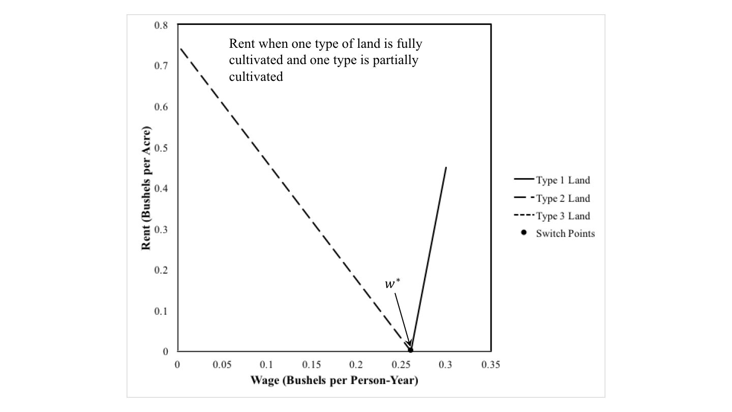
Suppose the wage is taken as given. For a low wage, between zero and approximately 0.261 bushels per person-year, Type 2 land is the most fertile. Its wage curve lies on the outer envelope in Figure 2. So the Zeta technique will be adopted. On the other hand, consider a higher wage up to 3/10 bushels per person-year. The Delta technique, in which Type 1 land is fully cultivated and Type 2 land is partially cultivated, is cost-minimizing.

The same techniques are cost-minimizing, under these assumptions about requirements for use, if the rate of profits is taken as given. For a low rate of profits, below approximately 62 percent, the Delta technique is cost minimizing. For a higher rate of profits, up to 100 percent, farmers will adopt the Zeta technique.

Figure 3 graphs rent against the wage. When the Zeta technique is operated, Type 2 land is fully cultivated and is the only type of land that pays a rent. The analogous conclusion holds for Type 1 land. The rate of profits increases to the left in the figure.

Figure 3: Rent When Two Types of Land are Taken In Cultivation

The assumption, in this example, that only one land is fully cultivated illustrates the dependence of the order of fertility on distribution. It does not allow, however, one to contrast the importance of whether the wage or the rate of profits is taken as given. Nor does it illustrate the difference between the order of fertility and the order of rentability.

3.2 Two Types of Land Fully Cultivated, One Partially Farmed

Accordingly, suppose requirements for use are such that more than two types of land must be cultivated. Which type of land is partially farmed can be determined by looking at the inner envelope of the wage curves in Figure 2. Given the wage, the order of fertility, from most fertile to least fertile, is Type 2, Type 1, and Type 3 lands. The switch point occurs at a wage exceeding the maximum wage when Type 3 lands pay no rent.

Figure 4 graphs rent versus the wage in this case. For low wages, the order of rentability, from Type 2 to Type 1 to Type 3 lands, matches the order of rentability. For high wages, the order of rentability is Type 1, Type 2, Type 3. The order of rentability no longer matches the order of fertability.

Figure 4: Rent When Three Types of Land are Taken In Cultivation

By constrast, suppose the rate of profits is taken as given. For low rates of profits, the order of fertility is Type 1, Type 2, Type 3. For high rates of profits, it is Type 2, Type 1, Type 3. Figure 5 graphs the rent per acre, in this case, against the rate of profits. I also indicate the location of the switch point for wage curves on this graph. The order of rentability matches the order of fertility for low and high rates of profits, but not for intermediate rates of profits.

Figure 5: Another View of Rent When Three Types of Land are Taken In Cultivation

4.0 Partition of Part of the Parameter Space

I now do my usual thing of partitioning some selection of the parameter space. See Figure 1 at the top of this post. In each numbered region, the analysis of the choice of technique does not change, in some sense. Table 3 provides a brief characterization of each region, with perturbations in the given wage.

Table 3: Description of Partitions with Wage Given

Region	Wage	Rents	Technique	Summary
1	0 < w < w*	ρ1 = ρ2 = ρ3 = 0	Lambda	Type 2 partially farmed. Types 1 and 3 fallow.
	w* < w < wmax, 1	ρ1 = ρ2 = ρ3 = 0	Kappa	Type 1 partially farmed. Types 2 and 3 fallow.
2	0 < w < w*	ρ1 = ρ2 = ρ3 = 0	Lambda	Type 2 partially farmed. Types 1 and 3 fallow.
	w* < w < wmax, 2	ρ1 > 0. ρ2 = ρ3 = 0	Delta	Type 1 fully farmed. Type 2 partially farmed. Type 3 fallow.
3	0 < w < w*	ρ2 > 0. ρ1 = ρ3 = 0	Zeta	Type 2 fully farmed. Type 1 partially farmed. Type 3 fallow.
	w* < w < wmax, 2	ρ1 > 0. ρ2 = ρ3 = 0	Delta	Type 1 fully farmed. Type 2 partially farmed. Type 3 fallow.
4	0 < w < w1	ρ2 > ρ1 > 0. ρ3 = 0	Alpha	Order of rentability matches order of fertility, given wage.
	w1 < w < wmax, 3	ρ1 > ρ2 > 0. ρ3 = 0	Alpha	Order of rentability differs from order of fertility, given wage.

Section 3 emphasizes that how the choice of technique is analyzed depends on whether or not the wage or the rate of profits is taken as given. Table 4 describes the regions in Figure 1, assuming the rate of profits is given. The interesting aspect of these tables comes from contrasting the description of Region 4 in Tables 3 and 4.

Table 4: Description of Partitions with Rate of Profits Given

Region	Rate of Profits	Rents	Technique	Summary
1	0 < r < r*	ρ1 = ρ2 = ρ3 = 0	Kappa	Type 1 partially farmed. Types 2 and 3 fallow.
	r* < r < rmax, 2	ρ1 = ρ2 = ρ3 = 0	Lambda	Type 2 partially farmed. Types 1 and 3 fallow.
2	0 < r < r*	ρ1 > 0. ρ2 = ρ3 = 0	Delta	Type 1 fully farmed. Type 2 partially farmed. Type 3 fallow.
	r* < r < rmax, 2	ρ1 = ρ2 = ρ3 = 0	Lambda	Type 2 partially farmed. Types 1 and 3 fallow.
3	0 < r < r*	ρ1 > 0. ρ2 = ρ3 = 0	Delta	Type 1 fully farmed. Type 2 partially farmed. Type 3 fallow.
	r* < r < rmax, 1	ρ2 > 0. ρ1 = ρ3 = 0	Zeta	Type 2 fully farmed. Type 1 partially farmed. Type 3 fallow.
4	0 < r < r1	ρ1 > ρ2 > 0. ρ3 = 0	Alpha	Order of rentability matches order of fertility, given rate of profits.
	r1 < r < r*	ρ2 > ρ1 > 0. ρ3 = 0	Alpha	Order of rentability differs from order of fertility, given rate of profits.
	r* < r < rmax, 3	ρ2 > ρ1 > 0. ρ3 = 0	Alpha	Order of rentability matches order of fertility, given rate of profits.

5.0 Conclusion

This post is not about what is wrong with aggregating capital. Nor is it about aggregate production functions. It is an exploration of an open model, and this model is therefore not a marginalist general equilibrium model. It synthesizes some ideas in Sraffa (1925) and Sraffa (1960). I think especially of Sraffa's comments on Wicksteed's distinction between descriptive and functional curves, between spurious and genuine margins.

References

• Piero Sraffa. 1925. Relazioni fra costo e quantita prodotta. Annali di Economia 2. Trans. by A. Roncaglia and J. Eatwell.
• Piero Sraffa. 1960 The Production of Commodities by Means of Commodities Cambridge University Press.
• J. E. Woods. 1990. The Production of Commodities: An Introduction to Sraffa. Atlantic Highlands: Humanities Press.